Comparison
L1 vs L2 vs Elastic Net
Understanding the different ways to regularize models by adding penalties to the loss function.
Verdict: Use L1 for feature selection (sparsity). Use L2 to shrink all weights smoothly. Use Elastic Net to get both.
Quick Version (TL;DR)
Understanding the different ways to regularize models by adding penalties to the loss function.
The Short Answer
Regularization prevents overfitting by penalizing a model for having large weights. It adds a "cost" to the loss function based on the size of the weights.
- L1 (Lasso) adds a penalty equal to the absolute value of the weights. It forces many weights to become exactly zero, effectively acting as a feature selector.
- L2 (Ridge) adds a penalty equal to the square of the weights. It shrinks all weights towards zero, but almost never makes them exactly zero.
- Elastic Net is simply a combination of both L1 and L2 penalties.
Where They Differ
| Feature | L1 (Lasso) | L2 (Ridge) | Elastic Net |
|---|---|---|---|
| Penalty Term | (Absolute value) | (Squared value) | |
| Geometric Shape | Diamond (sharp corners) | Circle (smooth edges) | "Squircle" (sharp corners, curved edges) |
| Produces Sparsity? | Yes. Drives irrelevant weights to exactly 0. | No. Weights get very small, but rarely 0. | Yes. |
| Handling Correlated Features | Arbitrarily picks one feature and ignores the rest. | Shrinks them together (keeps them all). | Keeps groups of correlated features together. |
| Computation | Harder (non-differentiable at 0). | Easier (smooth and differentiable). | Moderate. |
The Geometric Explanation
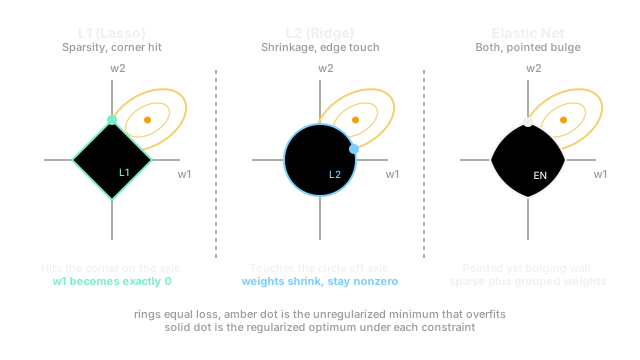
If you look at the visual diagram, you'll see why L1 creates zeros and L2 doesn't.
Imagine the unregularized loss as a bowl (the red contours). We want to find the lowest point in the bowl, but regularization places a fence around the origin (0,0) and says "you cannot step outside this fence."
- L2's fence is a circle. When the bowl's contours expand and hit the circle, they almost always hit it on a curve, meaning both and will have non-zero values.
- L1's fence is a diamond. Diamonds have sharp corners that lie exactly on the axes. When the bowl expands, it is highly likely to hit a sharp corner first. If it hits the corner on the y-axis, then the x-axis weight () is exactly zero.
Choose L1 (Lasso) When
- You need feature selection: You have 10,000 features (e.g., genes) and you want the model to tell you the 10 that actually matter.
- Interpretability is critical: A model with 5 non-zero weights is much easier to explain to a stakeholder than a model with 1,000 tiny weights.
Choose L2 (Ridge) When
- You have highly correlated features: L2 will distribute the weight among all correlated features rather than arbitrarily dropping some.
- You don't need sparsity: If you believe all your features contribute slightly to the target, L2 is usually the best default choice. Deep neural networks almost exclusively use L2 regularization (often called "weight decay").
Choose Elastic Net When
- You have correlated features AND you want sparsity: L1 struggles when features are highly correlated (it randomly drops one). Elastic net solves this by using the L2 penalty to group correlated features, and the L1 penalty to select or drop the entire group together.
What People Get Wrong
Assuming Regularization is only for Linear Models
While Lasso and Ridge are technically specific linear regression models, the penalties (L1 and L2) are used everywhere. L2 regularization is a fundamental component of training almost every modern deep learning model to prevent the network from memorizing the training data.