Core ML

Convolutional Neural Networks

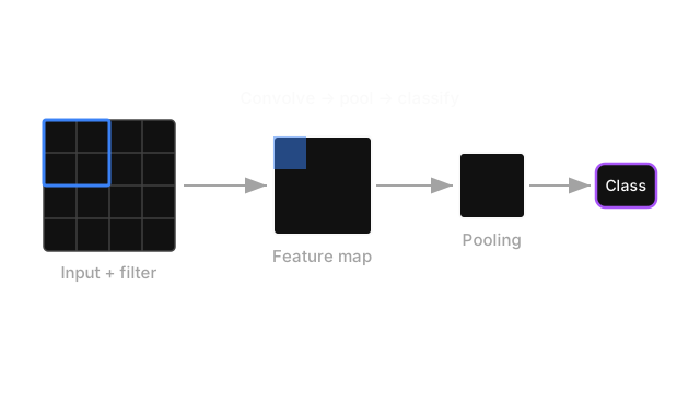
Stack convolution, activation, and pooling, then read out with a classifier — the architecture that made raw pixels a workable neural-network input.

A convolutional neural network alternates convolution and pooling to shrink the map while deepening its channels, then flattens what's left into a vector a classifier can read

Why Does This Exist?

Say the task is reading chest X-rays for signs of pneumonia — a hospital's radiology queue is backed up, and a first-pass triage model could flag the scans that most need a doctor's attention today. The input is a 28×28 grayscale crop around the lungs. A pneumonia-related opacity might be a faint cloudiness spanning forty pixels in one image and fifteen in another, in a different location each time, at a different scale each time.

That's three separate problems for one model to solve at once: recognize a pattern (the texture of an opacity), recognize it anywhere in the frame (a lung's edges aren't centered the same way for every patient), and recognize it whatever its extent (early versus advanced). No single tool solves all three. Convolution solves the first — a shared kernel that detects a pattern wherever it appears. Pooling contributes to the second, some tolerance to exactly where a signal sits. Depth, and the receptive field it grows, solves the third — a deep unit's field widens layer by layer until it can span a large opacity, not just a small one.

A convolutional neural network is the architecture that combines all three, in a specific repeating shape, and then adds one more piece: a way to turn "here's a map of where patterns fired" into "here's a single answer." That's the whole page.

Think of It Like This

A radiologist's reading, step by step

A radiologist doesn't examine every pixel of an X-ray in isolation, and they don't jump straight to a verdict either. They scan for small local signs first — an edge here, a density difference there. Then they step back and look at how those small signs group into regions: is this cloudiness confined to one lobe, or does it span both lungs? Only after building up from small signs to larger regions do they commit to a diagnosis.

A CNN runs the same escalation, mechanically. Early layers detect small local patterns — edges, simple textures — because their kernels are tiny and their receptive fields are narrow. Later layers, reading the output of earlier ones rather than raw pixels, respond to larger, more composite patterns built from those small signs. The final layer takes whatever the deepest layer settled on and turns it into one decision.

How It Actually Works

The repeating block

A CNN's body is built from one repeating unit: a convolutional layer, an activation function, then usually a pooling layer. Convolution detects a set of patterns and produces one feature map per kernel — a stack of channels, not a single image anymore. An activation function — ReLU is the standard choice here — introduces the nonlinearity that keeps stacking these blocks from collapsing into one big linear operation. Pooling then shrinks the spatial dimensions, trading resolution for both compute savings and some tolerance to exact position.

Trace the X-ray through two such blocks and the shape changes concretely: the 28×28×1 input becomes 14×14×8 after the first conv-and-pool pass, then 7×7×16 after the second — spatial size shrinking by half each time, channel count growing each time. That's the general pattern: width and height shrink with depth, channel count grows with depth. Early layers hold a lot of spatial detail and few channels; late layers hold little spatial detail and many channels, because by then the network has traded "where, precisely" for "what, more richly described."

From a grid of numbers to a single decision

Everything up to this point produces a 3D block of numbers — height, width, channels. A classification decision needs a fixed-length vector, so somewhere the network has to collapse the spatial dimensions away. Flattening does this by the simplest possible route: unroll the whole 7×7×16 block into one long vector, in this trace, 784 numbers, with no operation performed, just a reshape.

That flattened vector then feeds one or more fully-connected layers — the same kind of layer a plain multi-layer perceptron is built from — ending in an output layer sized to the number of classes. For pneumonia-or-not, that's two numbers, turned into a probability by a final softmax or sigmoid. Everything before flattening is convolutional and translation-shared; everything after is fully connected and, for the first time in the network, has weights specific to where in the flattened vector a value sits.

Every kernel learns its own pattern

Nothing hand-designs what an early kernel looks for. Every one of a layer's kernels starts from random weights and updates through the same backpropagated gradient every other weight in the network gets. What consistently emerges, across wildly different training runs and datasets, is a predictable hierarchy: the earliest layer's kernels converge on simple edge and color-contrast detectors, middle layers converge on textures and simple shapes, and later layers respond to compositions specific to the training data — a particular kind of opacity, in this case, rather than a generic "texture." Nobody wrote a rule that says "first layer, detect edges." The architecture's structure — small kernels near the input, larger effective receptive fields deeper in — makes that division of labor the natural solution for gradient descent to find.

Show Me the Code

The exact shape trace from the prose above, computed rather than asserted, using only the arithmetic each layer performs on its input's dimensions.

1def conv_output(size: int, kernel: int, padding: int, stride: int) -> int:2    return (size + 2 * padding - kernel) // stride + 13
4
5def cnn_shape_trace(h: int, w: int, c: int) -> None:6    # Block 1: 3x3 conv, padding 1 (keeps size), 8 filters -> then 2x2 pool, stride 27    h, w, c = conv_output(h, 3, 1, 1), conv_output(w, 3, 1, 1), 88    h, w = h // 2, w // 29    print(f"after block 1: {h}x{w}x{c}")10
11    # Block 2: 3x3 conv, padding 1, 16 filters -> then 2x2 pool, stride 212    h, w, c = conv_output(h, 3, 1, 1), conv_output(w, 3, 1, 1), 1613    h, w = h // 2, w // 214    print(f"after block 2: {h}x{w}x{c}")15
16    flat = h * w * c17    print(f"flattened length: {flat}")  # what the fully-connected head actually receives18
19
20cnn_shape_trace(h=28, w=28, c=1)21# -> after block 1: 14x14x822# -> after block 2: 7x7x1623# -> flattened length: 784

Every number here matches the diagram directly. The flattened length is the one figure that's easy to get wrong by hand when designing a network's fully-connected head — computing it, rather than guessing, is the difference between a shape error at the first training step and a network that runs.

Watch Out For

A shape mismatch at the flatten step that only surfaces at runtime

The single most common first-time error building a CNN by hand is hardcoding the flattened vector's length — writing Linear(1568, num_classes) because that's what worked for a 32×32 input, then feeding the network a 28×28 image and watching it crash at the first forward pass with a matrix-shape error that names two numbers and no obvious cause.

The fix is the trace above: compute the spatial size after every conv and pool layer explicitly, given your actual input size, rather than assuming it. Most frameworks also offer a way to run one dummy forward pass and read the resulting shape directly, which sidesteps hand arithmetic entirely and is worth doing before writing the fully-connected head at all.

Pooling and downsampling too aggressively for the input's real size

Two or three pooling layers on a 28×28 input is fine — the trace above ends at a still-meaningful 7×7. Apply the same architecture, unmodified, to a much smaller crop, and repeated halving can shrink the spatial dimensions to 1×1 or even try to go below it, discarding essentially all spatial structure before the network has had a chance to use it, or erroring outright.

Match the depth of downsampling to the input size, and check the spatial dimensions at each stage rather than assuming an architecture that worked for one input size transfers unmodified to another.

The Quick Version

A CNN alternates convolution, activation, and pooling: convolution detects patterns and produces channels, activation adds nonlinearity, pooling shrinks the spatial map.
Spatial size shrinks with depth; channel count grows with depth — the network trades "where, precisely" for "what, more richly described."
Flattening reshapes the final 3D block into a vector with no computation, so a fully-connected head — ordinary dense layers — can turn it into a classification decision.
What each kernel learns to detect emerges from training, not design — early layers converge on edges and simple textures, later layers on compositions specific to the data.
Always compute the flattened vector's length from the actual input size and layer stack; hardcoding it is the most common first CNN bug.