Double Machine Learning (DML)

Why Does This Exist?

In classic causal inference (like Propensity Score Matching or basic Linear Regression), we assume the relationships between variables are simple, usually linear. But in the real world, confounders affect outcomes in highly complex, non-linear ways. Age might increase income up to age 50, then decrease it, and it might interact strongly with education level.

To capture this complexity, we want to use powerful algorithms like Random Forests, Gradient Boosting, or Neural Networks. However, standard ML models are fundamentally biased when it comes to causal inference. They use regularization (like L1/L2 penalties or tree pruning) to prevent overfitting. This regularization actively shrinks coefficients towards zero, which systematically biases your estimate of the treatment effect.

Double Machine Learning (DML) exists to allow you to use advanced, non-linear ML models for causal inference without suffering from regularization bias.

Think of It Like This

How It Actually Works

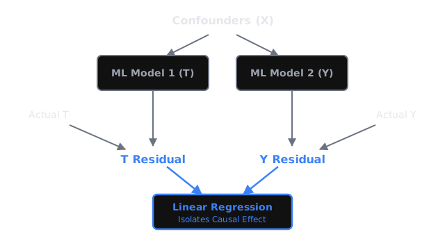
Double ML (formulated by Chernozhukov et al., 2018) relies on a mathematical trick called Orthogonalization (or the Frisch-Waugh-Lovell theorem). It works in three steps:

Step 1: Predict the Treatment (Model 1)

Train an ML model (e.g., LightGBM) to predict who receives the Treatment ($T$) based on the confounders ($X$). Subtract the model's prediction from the actual treatment to get the Treatment Residual ($\tilde{T} = T - \hat{T}$). This residual represents the totally random, unexplained variation in the treatment.

Step 2: Predict the Outcome (Model 2)

Train a completely separate ML model to predict the Outcome ($Y$) based on the confounders ($X$), completely ignoring the treatment. Subtract the model's prediction from the actual outcome to get the Outcome Residual ($\tilde{Y} = Y - \hat{Y}$). This residual represents the totally random, unexplained variation in the outcome.

Step 3: The Causal Regression

Run a simple, un-regularized Linear Regression predicting the Outcome Residuals using the Treatment Residuals: $\tilde{Y} \sim \tilde{T}$. Because both variables have been perfectly stripped of all the confounding noise from $X$, this simple regression yields the unbiased Average Treatment Effect (ATE).

To prevent overfitting from ruining the residuals, this entire process is done using Cross-Fitting (similar to k-fold cross-validation), ensuring that the model predicting a user's outcome was never trained on that user's data.

Show Me the Code

You don't have to code the residual math manually. Microsoft's EconML library handles the cross-fitting and residualization for you.

1import numpy as np2import pandas as pd3from lightgbm import LGBMRegressor, LGBMClassifier4from econml.dml import LinearDML5
6# X: Complex, high-dimensional confounders7# T: Treatment (0 or 1)8# Y: Outcome9
10# 1. Initialize the Double ML estimator11# We use LightGBM to model the complex nuisance parameters12est = LinearDML(13    model_y=LGBMRegressor(n_estimators=100, max_depth=3), # Predicts Outcome14    model_t=LGBMClassifier(n_estimators=100, max_depth=3), # Predicts Treatment15    discrete_treatment=True,16    cv=5, # 5-fold cross-fitting to prevent overfitting17    random_state=4218)19
20# 2. Fit the model21# EconML automatically handles the orthogonalization and residual regression under the hood22est.fit(Y, T, X=X)23
24# 3. Get the Causal Effect25ate = est.ate(X)26print(f"Estimated Average Treatment Effect: {ate:.3f}")27
28# You can also get valid confidence intervals and p-values!29summary = est.summary()30print(summary)

Watch Out For

The Quick Version

• Standard ML algorithms (like Random Forests) are inherently biased for causal inference because of regularization.
• Double Machine Learning (DML) fixes this by using ML strictly to model the "nuisance" variables (the confounders).
• It trains two models: one predicting Treatment, one predicting Outcome.
• By subtracting these predictions, we create residuals that are completely orthogonal to the confounders.
• Regressing the Outcome residuals on the Treatment residuals gives an unbiased, highly accurate causal effect.

What to Read Next

• heterogeneous-treatment-effects — How to use the exact same Double ML architecture to find out who was affected most by the treatment, rather than just the average.
• uplift-modeling — How to turn Causal ML into a ranking problem for marketing and sales optimization.
• propensity-score-methods — Review the older, less robust method of handling observational data.