Core ML

Generative Adversarial Networks

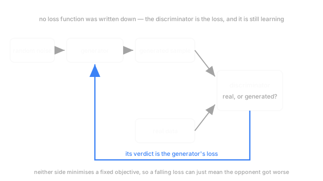
Nobody writes the loss. A second network learns to spot fakes, and the generator's only job is to fool it, which makes it a game rather than a minimisation.

Two paths reach one discriminator, real data on the lower and generated samples on the upper, and its verdict is the only training signal either network ever gets

Why Does This Exist?

A rolling mill inspects steel sheet with a line camera and wants a model that flags surface defects. Defects are the problem: 40,000 photographs of clean sheet, 300 of scratches, pits and roll marks. Nobody is going to damage good steel to get more.

So generate them. And here the obvious approach stops dead. Every model on this site so far minimises a loss you wrote down, and there's no expression for this photograph looks like a real roll mark. Squared error against a real defect gives the average of all defects, a grey smudge — it's a claim about how errors are distributed, and no such claim describes photographic realism.

The idea, from 2014, is to stop writing the loss and learn one. Put a second network in charge of judging real against generated, and make the first network's objective that network's failure rate. The judge improves, the standard rises, the generator improves, the judge improves again.

Two names. The generator maps random noise to an image. The discriminator takes an image and outputs how real it thinks it is.

Think of It Like This

A forger and an auctioneer who both keep getting better

A forger paints a canvas and hands it to an auctioneer who has to say real or fake. Early on the auctioneer only checks the signature, so a passable signature is enough and the forger learns nothing about paint.

Then the auctioneer checks the craquelure. Signatures no longer help; the forger has to learn how old varnish cracks. Then pigment chemistry, then brush pressure at the edges. Every new tell moves the forger's target, and every closed gap forces a harder one.

Nobody ever wrote down what a real painting is. The standard was built by two people disagreeing.

The failure is in the story too. If the forger finds one canvas the auctioneer keeps passing, painting that canvas forever is the sensible move. It works, and it's useless to a gallery that wanted a collection.

How It Actually Works

A game, not a minimisation

The discriminator is trained on an ordinary classification loss: real photographs labelled real, generated ones fake. The generator is trained to make that loss worse. One objective, two players pulling opposite ways, which is why this is a minimax problem rather than a minimisation.

The consequence matters more than the algebra: neither network's loss is a progress measure. Normally a falling loss means the model improved. Here it can equally mean the discriminator got worse. The two numbers describe a relationship, so they say almost nothing about sample quality — which breaks every habit built on a loss curve, including how you pick a checkpoint.

Implicit density, and what that buys and costs

A variational autoencoder optimises a bound on the likelihood of the data, so it has an explicit density: approximate, but you can ask it how probable a given image is. A GAN never writes a probability down anywhere. It has a sampler and nothing else, and that is what implicit means.

Which explains the trade practitioners feel. No density means no averaging over plausible outputs, so GAN samples are sharp where a VAE's are soft — the whole reason they took over image synthesis. It also means no score for a held-out image, no likelihood, and no principled convergence criterion.

The three failures

Mode collapse is the signature one, and the forger's canvas is exactly it. The generator finds a narrow set of outputs the current discriminator won't reject and produces only those. Samples look excellent, diversity is gone. Your defect generator emits one convincing scratch thousands of times, and a detector trained on it has learned one scratch.

Non-convergence. Two networks chasing each other can cycle indefinitely without settling, and no loss value tells you which part of the cycle you're in.

Vanishing generator gradient. If the discriminator gets far ahead early it rejects every generated image with near-total confidence, and a confident correct answer carries almost no gradient — so the generator gets nothing to act on exactly when it needs direction.

The stabilisers come in three families: objectives that keep supplying usable gradient while the discriminator wins, constraints that stop it becoming too sharp, and schedules that build resolution or capacity gradually.

Show Me the Code

No networks. Just the measurement that catches mode collapse, and the measurement that misses it.

1import numpy as np2
3rng = np.random.default_rng(3)4MODES = np.array([-6.0, -2.0, 2.0, 6.0])  # four kinds of defect the mill actually sees5
6
7def realism(x: np.ndarray) -> float:8    d = np.exp(-0.5 * ((x[:, None] - MODES) / 0.4) ** 2).sum(axis=1)9    return float(np.log(d + 1e-12).mean())  # how plausible each sample is on its own10
11
12def modes_hit(x: np.ndarray) -> int:13    nearest = np.abs(x[:, None] - MODES).argmin(axis=1)14    return int(len(np.unique(nearest[np.abs(x - MODES[nearest]) < 1.2])))15
16
17real = rng.choice(MODES, 4000) + rng.normal(0.0, 0.4, 4000)18collapsed = MODES[1] + rng.normal(0.0, 0.4, 4000)  # one defect type, over and over19covering = rng.choice(MODES, 4000) + rng.normal(0.0, 0.4, 4000)20for name, s in (("real data", real), ("collapsed", collapsed), ("covering", covering)):21    print(f"{name:10s} realism {realism(s):+.3f}   modes hit {modes_hit(s)} of 4")22# -> real data  realism -0.511   modes hit 4 of 423# -> collapsed  realism -0.503   modes hit 1 of 424# -> covering   realism -0.474   modes hit 4 of 4

The collapsed generator scores −0.503 on realism, marginally better than real data's −0.511, because every sample sits dead centre of a real mode. Per-sample plausibility cannot see the failure. Coverage sees it immediately: one mode of four.

Watch Out For

Mode collapse read as success because the samples look good

Somebody generates a sheet of sixty defect images, they look convincing, and the model ships. Two weeks later the detector catches scratches beautifully and misses roll marks entirely, because roll marks were never in the set the generator produced.

Eyeballing a sample sheet measures per-image quality, exactly the axis collapse leaves intact. Measure diversity deliberately: cluster the generated samples and count how many clusters get used, or compare per-class counts against the real distribution when you have labels. Sixty images is also too small to notice — a generator emitting three distinct defects can fill sixty tiles and look varied.

Picking a checkpoint by the loss curve

The generator loss is at its lowest at step 40,000, so that checkpoint ships. Its samples are worse than the one from step 25,000.

In a two-player game a low generator loss means it's currently beating the discriminator, and the cheapest way to beat a weak discriminator is not to get better. The number describes who is ahead, not how good the samples are. So checkpoint selection has to come from outside the game: a sample-quality measure against real data, a diversity measure beside it, human inspection of a big enough sheet. This costs more than reading a curve.

The Quick Version

No loss is written down. A discriminator learns one, and the generator's objective is that discriminator's failure.
Two players with opposed objectives, so it's a game. Neither loss measures progress: a falling generator loss can just mean the opponent weakened.
Implicit density: a sampler and nothing else. That buys sharpness and costs likelihoods and any convergence criterion.
Mode collapse is the signature failure — narrow output the discriminator can't reject, so quality holds while diversity dies.
Non-convergence and a vanishing generator gradient are the other two, the second when the discriminator gets too far ahead too early.
Per-sample realism can't detect collapse. Measure coverage separately, and select checkpoints on sample quality, not loss.