Core ML

Gradient Accumulation

Run several small forward-backward passes and sum their gradients before one optimizer step, so limited GPU memory can still train as if it saw one large batch.

Four small micro-batches run one after another, each contributing its gradient to a running sum, until one optimizer step fires using the combined total — the same update one large batch would have produced

Why Does This Exist?

A model and its activations for one training batch have to fit in GPU memory at the same time — the weights, the intermediate values saved for backpropagation, and the batch of inputs all compete for the same fixed pool. Batch size effects explains why a specific batch size might genuinely be the right one for training stability or throughput, but "the batch size the recipe calls for" and "the batch size that fits in memory" are two different numbers, and the second is often smaller. Buying a bigger GPU is one answer. Gradient accumulation is the answer that doesn't require new hardware at all.

Think of It Like This

Filling a bucket with a cup

A recipe calls for one full bucket of water added to a mix all at once, but all you have is a small cup — the bucket itself is too heavy to carry full. The fix isn't to give up on the recipe's proportions; it's to carry cup after cup over to the mix, keeping count, and only stir the mix in once the running total actually equals a full bucket.

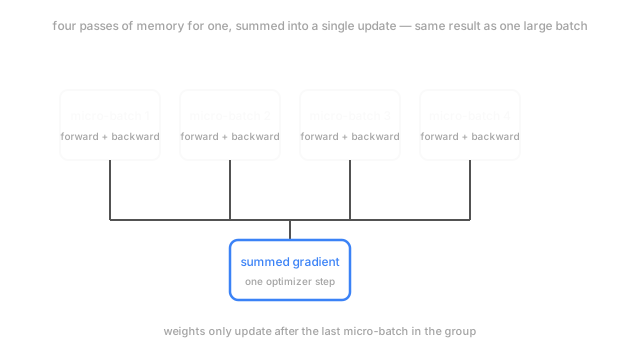
Gradient accumulation is the same move: run several small forward-backward passes, each computing a gradient the memory budget can actually hold, and add each one into a running total. Only once that total represents the full intended batch does the optimizer actually update the weights — the mix only gets stirred once, at the right moment, using the full amount.

How It Actually Works

The accumulation loop

For $K$ micro-batches meant to simulate one batch of the target size, the loop runs the forward and backward pass on each micro-batch, letting the gradients add into the same buffer instead of clearing it between micro-batches, and only calls the optimizer step after the $K$ -th one:

1zero the gradient buffer2for i in 1..K:3    forward pass on micro-batch i4    backward pass, gradients add into the buffer5    (do not zero the buffer, do not step the optimizer)6divide the accumulated gradient by K7optimizer step using the accumulated, averaged gradient

Only one micro-batch's activations are ever in memory at once — the model runs $K$ separate forward-backward passes, each cheap in memory, rather than one pass over a batch $K$ times larger. What's expensive to hold in memory (activations for the full batch) is traded for something cheap to hold (one running gradient sum, the same size as the model's parameters).

Why the result is (nearly) the same as a real large batch

A large batch's gradient is the average of its examples' individual gradients. Summing $K$ micro-batches' gradients and dividing by $K$ computes exactly that same average, just accumulated in pieces rather than all at once — the arithmetic is identical, not an approximation. What differs slightly in practice is anything that depends on seeing the whole batch simultaneously, most notably batch normalization: normalizing each micro-batch's statistics separately isn't the same as normalizing over the full combined batch, which is why gradient accumulation is commonly paired with layer normalization or group normalization instead when this matters.

What accumulation does and doesn't buy

It reproduces a large batch's gradient estimate, at the cost of $K$ times the wall-clock time compared to genuinely running the full batch at once on hardware big enough to hold it — there's no free compute here, only a memory-for-time trade. It's the standard technique for reaching a target effective batch size on hardware that can't fit that batch directly, and it composes with mixed precision training, which is the other major lever for the same underlying memory constraint.

Show Me the Code

Accumulating gradients over four micro-batches produces the exact same result as computing the gradient over the full batch at once.

1import numpy as np2
3rng = np.random.default_rng(1)4data = rng.normal(0, 1, size=(16, 4))  # 16 examples, 4-dim gradient contribution each5
6large_batch_grad = data.mean(axis=0)7
8micro_batches = data.reshape(4, 4, 4)  # 4 micro-batches of 4 examples9accumulated_grad = np.mean([mb.mean(axis=0) for mb in micro_batches], axis=0)10
11print(f"large batch: {np.round(large_batch_grad, 4)}")12print(f"accumulated: {np.round(accumulated_grad, 4)}")13print(f"match: {np.allclose(large_batch_grad, accumulated_grad)}")14# -> large batch: [-0.0934 -0.0244  0.0964 -0.272 ]15# -> accumulated: [-0.0934 -0.0244  0.0964 -0.272 ]16# -> match: True

The two gradients are identical, not merely close — accumulation and averaging is exact arithmetic, not an approximation of a large-batch gradient.

Watch Out For

Forgetting to divide the accumulated gradient by the number of micro-batches

Summing $K$ micro-batch gradients without dividing by $K$ before the optimizer step produces a gradient roughly $K$ times too large, which behaves like a learning rate spike — training destabilizes in a way that looks like a bad learning rate choice but is actually a missing division in the accumulation loop.

Using batch normalization unmodified across accumulation steps

Batch normalization computes statistics from the batch it's given — a micro-batch's mean and variance are not the full batch's mean and variance, so normalizing per-micro-batch changes what the layer actually does compared to running the full batch through it directly. This is the reason layer or group normalization is the more common pairing with gradient accumulation in practice.

The Quick Version

GPU memory limits the batch size that fits in one forward-backward pass; gradient accumulation gets around that limit without new hardware.
Several small micro-batches run in sequence, each adding its gradient into a shared buffer instead of triggering an optimizer step.
After $K$ micro-batches, the summed gradient is divided by $K$ and one optimizer step runs — arithmetically identical to averaging over one real batch of that size.
The trade is wall-clock time for memory: $K$ sequential passes cost roughly $K$ times the time a single large-batch pass would.
Batch normalization doesn't accumulate cleanly across micro-batches; layer or group normalization is the more common pairing.