Core ML

ML Pipeline Architecture

A Jupyter Notebook is not software. An ML Pipeline turns a messy, manual research script into a repeatable, automated factory that ingests data and produces deployable models.

An ML Pipeline is a Directed Acyclic Graph (DAG) of discrete steps. Data flows strictly from left to right: Ingestion -> Preprocessing -> Training -> Evaluation -> Registry.

Why Does This Exist?

In the beginning, a Data Scientist writes a Jupyter Notebook. They download a CSV, clean the null values, train an XGBoost model, print the accuracy, and save the model file to their desktop.

This works for a hackathon, but it is a disaster for a company. What happens next month when the data changes and the model needs retraining? Does the Data Scientist just run the notebook again? What if they left the company? What if the notebook only runs on their specific laptop because of a weird dependency?

An ML Pipeline solves this by converting the machine learning process from a manual craft into an automated factory. It breaks the notebook into distinct, repeatable code steps that run on a schedule in the cloud.

Think of It Like This

Imagine a master chef baking a cake. They taste the batter, add a little extra sugar intuitively, and bake it until it "looks right." That is a Jupyter Notebook. It produces a great cake once, but nobody else can replicate it.

Now imagine a commercial bakery. There are separate, automated stations: Station 1 measures exact flour. Station 2 mixes for exactly 4 minutes. Station 3 bakes at exactly 350°F. If the cake comes out bad, you know exactly which station failed. That is an ML Pipeline.

How It Actually Works

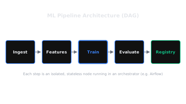
An ML Pipeline is structurally a Directed Acyclic Graph (DAG). It is a sequence of isolated scripts (Nodes) connected by data dependencies (Edges). It typically consists of 5 core stages:

1. Data Ingestion

The pipeline wakes up (e.g., triggered by a cron job every Sunday at midnight). It reaches into the data warehouse (Snowflake, BigQuery), runs a SQL query to pull the last 30 days of user behavior, and saves it to cloud storage (S3).

2. Feature Engineering & Preprocessing

The pipeline reads the raw data from S3. It imputes missing values, normalizes numerical columns, and one-hot encodes categorical variables. Crucially, it saves these preprocessing parameters (like the mean and variance used for scaling) so they can be reused at inference time.

3. Model Training

The pipeline spins up a GPU machine. It downloads the preprocessed data and trains the model (e.g., a PyTorch network). It tracks hyperparameters and loss curves using an Experiment Tracker (like MLflow or Weights & Biases).

4. Model Evaluation

Before anyone uses the model, the pipeline tests it against a holdout validation set. It calculates metrics (Accuracy, F1-Score, RMSE). If the new model performs worse than the model currently in production, the pipeline halts immediately.

5. Model Registration

If the model passes evaluation, the pipeline packages the model weights, the preprocessing parameters, and the dependencies into a single artifact and uploads it to a Model Registry. It is now ready for deployment.

Show Me the Code

In modern ML engineering, pipelines are written using orchestration frameworks like Airflow, Kubeflow, or Prefect. Here is a conceptual example using a Python-based orchestrator (similar to Prefect).

1from prefect import task, flow2import pandas as pd3
4# Define the isolated steps (Tasks)5@task6def extract_data():7    return pd.read_csv("s3://bucket/raw_data.csv")8
9@task10def clean_data(df):11    return df.fillna(0)12
13@task14def train_model(df):15    from sklearn.ensemble import RandomForestClassifier16    model = RandomForestClassifier().fit(df[['X']], df['y'])17    return model18
19@task20def evaluate_and_register(model, df):21    score = model.score(df[['X']], df['y'])22    if score > 0.85:23        print(f"Model passed with {score}. Registering!")24        # mlflow.register_model(...)25    else:26        raise ValueError("Model degraded. Halting pipeline.")27
28# Define the DAG (Flow)29@flow(name="Weekly-Churn-Model-Pipeline")30def ml_pipeline():31    # The pipeline logic explicitly defines the Directed Acyclic Graph (DAG)32    raw_data = extract_data()33    clean_data = clean_data(raw_data)34    model = train_model(clean_data)35    evaluate_and_register(model, clean_data)36
37# Run the pipeline38if __name__ == "__main__":39    ml_pipeline()

Watch Out For

The "Hidden State" Trap. The most common mistake when converting a notebook to a pipeline is leaving "hidden state." In a notebook, if you run Cell 4, then Cell 2, then Cell 5, your model depends on that exact, invisible execution order. In a pipeline, every single step must be perfectly isolated and stateless. A step should only know about the data passed directly into it via its function arguments.

The Quick Version

A Jupyter Notebook is manual and unrepeatable. An ML Pipeline is automated and repeatable.
Pipelines are modeled as DAGs (Directed Acyclic Graphs) running on orchestrators like Airflow or Kubeflow.
The standard pipeline stages are: Ingest $\rightarrow$ Preprocess $\rightarrow$ Train $\rightarrow$ Evaluate $\rightarrow$ Register.
If a pipeline fails at the Evaluation stage, it halts to prevent a degraded model from reaching production.