Core ML

Momentum

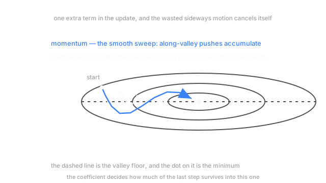
Plain descent zig-zags across a narrow valley. Average the last few gradients instead: the sideways pushes cancel and the downhill push keeps stacking up.

Why Does This Exist?

You want to get to the bottom of a loss surface, and you want to get there in fewer steps than you're currently taking. That's the whole goal.

Here's where the obvious approach stops working, on the example we'll keep coming back to. You're predicting a house's monthly heating bill from two features: floor area and number of rooms. Those two move together — bigger houses have more rooms — so the model can trade one against the other almost freely. Add a bit to the area coefficient, subtract a bit from the rooms coefficient, and the loss barely changes. The result is a loss surface shaped like a long narrow trough: steep across, nearly level along.

Now run plain gradient descent in that trough. The gradient at almost every point mostly points across the valley, toward the nearest wall, because that's the steep direction. Each step throws you at the far wall, the next throws you back, and the component that actually reduces the loss — the one along the floor — is a small fraction of every step. You zig-zag. Lower the learning rate and the zig-zag tightens but the crawl gets slower too. No setting fixes it.

Think of It Like This

A bobsled in a chute

A bobsled going down an ice chute. The chute is banked, so when the sled rides up one wall the ice pushes it back toward the middle, and a moment later the other wall pushes it the other way. Those pushes are opposite, and over a run they roughly cancel — the sled ends up going down the middle without anyone steering it there.

Gravity along the chute never reverses. Every metre adds to the same forward speed.

That's the split. Forces that flip sign cancel out of the motion; the force that keeps pointing one way becomes speed. A ball rolling in the trough of a loss surface does exactly this, which is why this method is also called the heavy ball.

How It Actually Works

Stop stepping along the current gradient. Keep a running total of recent gradients and step along that:

v_{t+1} = \beta v_t - \eta \nabla_\theta L(\theta_t), \qquad \theta_{t+1} = \theta_t + v_{t+1}

$v_t$ is the velocity, a vector the same shape as the parameters, starting at zero. $\beta$ is the momentum coefficient, between zero and one. $\eta$ is the learning rate and $\nabla_\theta L(\theta_t)$ the gradient of the loss with respect to the parameters. At $\beta = 0$ you get plain gradient descent back.

Now the part the metaphor hides. Take the across-valley direction, where the gradient alternates: plus four, minus four, plus four. With $\beta = 0.9$ and $\eta = 1$ , the velocity runs minus four, then plus 0.4, then minus 3.64, and stays bounded around three and a half. It never exceeds the single gradient that produced it, because each new term arrives opposing nine tenths of what was already there.

Now the along-valley direction, where the gradient is a steady plus 0.4 — a tenth the size. Velocity: minus 0.4, minus 0.76, minus 1.08, and it keeps climbing toward minus four. Same sign every step, so the terms add.

Ten times the gradient magnitude, and after eight steps the small consistent direction has produced comparable velocity. That inversion is the entire mechanism.

What the coefficient means

$\beta$ sets how long a gradient keeps affecting your steps. Each one decays by a factor of $\beta$ per step, so the effective window is about $1/(1-\beta)$ steps — ten at 0.9, a hundred at 0.99. It also multiplies your reach: at a steady gradient the velocity settles at $\eta/(1-\beta)$ , so 0.9 moves you ten times further per step than plain descent at the same learning rate. Hold that thought for the pitfalls.

Nesterov's version

The standard variant asks a sharper question. Your velocity is about to carry you somewhere; why measure the gradient where you are rather than where you're going? Nesterov momentum evaluates it at $\theta_t + \beta v_t$ , the point the velocity is already committed to. If the loss starts rising there, the correction lands in this step instead of the next, so overshoot gets damped a step earlier. Small change, usually helps a little.

What it cost

One more hyperparameter. One extra copy of every parameter in memory, which for a large model is real. And a failure mode plain descent doesn't have: enough accumulated velocity and you sail through a narrow minimum, then oscillate around it for a long time.

Show Me the Code

The two directions, side by side. The gradient sequences are stylised, the velocity arithmetic is exactly what an optimiser runs.

1import numpy as np2
3
4def velocity(grads: np.ndarray, beta: float = 0.9) -> np.ndarray:5    v, out = 0.0, np.empty(len(grads))6    for t, g in enumerate(grads):7        v = beta * v - float(g)      # last step's direction survives, scaled by beta8        out[t] = v9    return out10
11
12across: np.ndarray = np.tile([4.0, -4.0], 4)   # valley walls: sign flips every step13along: np.ndarray = np.full(8, 0.4)            # valley floor: same sign, ten times smaller14
15print("across ", np.round(velocity(across), 2))16print("along  ", np.round(velocity(along), 2))17# -> across  [-4.    0.4  -3.64  0.72 -3.35  0.99 -3.11  1.2 ]18# -> along   [-0.4  -0.76 -1.08 -1.38 -1.64 -1.87 -2.09 -2.28]

The across row still bounces between the magnitudes it started with. The along row has grown fivefold, heading for minus four — the limit $\eta/(1-\beta)$ predicts.

Watch Out For

Raising the coefficient and the learning rate in the same experiment

Symptom: you nudge momentum from 0.9 to 0.99 for a run that was training fine, and it diverges within a few hundred steps. The obvious suspect is whatever else changed in that commit.

Effective step size is roughly $\eta/(1-\beta)$ . Going from 0.9 to 0.99 takes the denominator from 0.1 to 0.01, so you multiplied your effective step by ten without touching the learning rate. Divide the rate by ten when you raise the coefficient that far. Treat momentum as part of the step size rather than a separate dial and this stops surprising you.

Momentum left on for a fine-tuning run

Symptom: you drop the learning rate to something tiny to make careful adjustments to an already-good model, and the loss gets worse over the first few hundred steps before recovering. The tiny rate was supposed to make that impossible.

Velocity carries history. Early steps, when the gradients were large and consistent, loaded up a velocity that keeps pushing for roughly $1/(1-\beta)$ steps after the gradient has gone quiet — straight past the narrow optimum you wanted to settle into. When you cut the rate hard, cut the coefficient too, or reset the velocity to zero at the switch. Most schedulers do neither for you.

The Quick Version

Plain descent in a narrow valley wastes most of every step going sideways, and no learning rate fixes it.
Keep a running average of past gradients — a velocity — and step along that instead of the raw gradient.
Across-valley components alternate sign and cancel. The along-valley component is consistent and accumulates. That's the whole trick.
$\beta$ of 0.9 means an effective window of about ten gradients and an effective step about ten times the learning rate.
Nesterov evaluates the gradient where the velocity is taking you, so overshoot corrections arrive a step earlier.
Cost: one hyperparameter, one extra copy of the parameters, and a new way to overshoot a narrow minimum.