Core ML

Multicollinearity

When two input features move almost identically, a regression splits credit between them almost arbitrarily — coefficients swing wildly, but predictions barely move.

Two nearly identical input features let a wide range of coefficient splits between them produce almost the same combined prediction, so individual coefficients swing wildly across resamples while predictions stay stable

Why Does This Exist?

An analyst fits a linear regression predicting house prices from square footage and number of rooms, expecting to report "each additional room adds roughly $X to the price." The fitted coefficient for rooms comes back negative — more rooms, lower predicted price — which makes no sense and doesn't match anything in the data when plotted directly. Refit the same model on a slightly different sample of the same houses and the room coefficient flips positive and changes magnitude by a factor of five. The model's actual price predictions, meanwhile, barely move between the two fits.

Nothing is broken in the fitting procedure. Square footage and room count are highly correlated — bigger houses tend to have more rooms — and linear regression's coefficients answer a very specific question: how does the prediction change if this one feature moves while every other feature holds exactly still. When two features almost never vary independently in the data, that question has no stable answer, even though the combined prediction they produce together is perfectly stable.

Think of It Like This

Splitting credit between two people who always work together

Two employees have worked every single shift together for years, and management wants to know how much each one individually contributes to daily sales. Because they're never observed working separately, there's no way to isolate one's effect from the other's — a manager could credit all the value to employee A and none to employee B, or the reverse, or any split in between, and the combined sales total predicted for "both of them working" comes out identical either way.

Ask the same question with a slightly different set of shifts sampled, and the "individual credit" split can swing wildly — today it looks like A matters more, tomorrow's sample says B does — purely because the two have never been disentangled in the data. What's stable, in every version, is the prediction for the pair working together. Multicollinearity is exactly this: individual credit is unstable, combined effect is not.

How It Actually Works

Why coefficients become unstable while predictions don't

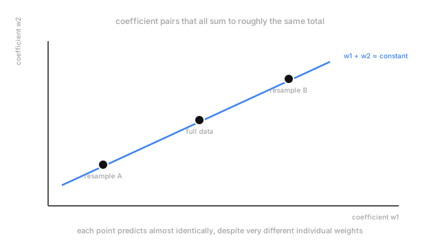
When two features $x_1$ and $x_2$ are nearly collinear — one is close to a linear function of the other — many different combinations of coefficients $w_1$ and $w_2$ produce almost the same value of $w_1 x_1 + w_2 x_2$ for every row in the data. The optimization has a long, nearly flat valley of almost-equally-good coefficient pairs to choose from, and which exact pair it lands on becomes extremely sensitive to small changes in the data — noise, or which specific sample you happened to draw. The sum $w_1 x_1 + w_2 x_2$ , which is what actually drives the prediction, stays essentially fixed even as the individual $w_1$ and $w_2$ swing across that valley.

The variance inflation factor: measuring it directly

The variance inflation factor (VIF) quantifies how much a coefficient's variance is inflated by collinearity with the other features. For feature $i$ , regress it on all the other features, take the resulting $R^2$ , and compute:

\text{VIF}_i = \frac{1}{1 - R_i^2}

A feature with $R^2 = 0$ against the others (no collinearity at all) gets VIF = 1 — no inflation. As $R_i^2$ approaches 1 — the feature becomes almost perfectly predictable from the others — VIF grows without bound. VIF values above roughly 5 to 10 are the commonly cited threshold for flagging a real problem, though the right cutoff depends on how much the specific analysis actually leans on interpreting individual coefficients.

Why this often doesn't matter, and when it does

If the goal is prediction accuracy alone, multicollinearity is frequently a non-issue — as shown directly below, predictions stay stable even while coefficients swing wildly, so a model used purely to generate forecasts can tolerate high VIF without any real cost. It becomes a genuine problem the moment anyone tries to interpret an individual coefficient: "each additional room is worth $X" is a claim about isolated effect, and multicollinearity is precisely the situation where that isolated effect cannot be estimated reliably from the data at hand, regardless of how large the dataset is.

Show Me the Code

Two coefficients swinging wildly across resamples of the same near-duplicate features, while predictions barely move.

1import numpy as np2
3
4def fit_ols(X: np.ndarray, y: np.ndarray) -> np.ndarray:5    Xb = np.hstack([X, np.ones((len(X), 1))])6    w, *_ = np.linalg.lstsq(Xb, y, rcond=None)7    return w8
9
10rng = np.random.default_rng(0)11x1 = rng.normal(0, 1, 200)12x2 = x1 + rng.normal(0, 0.01, 200)  # near-duplicate of x113y = 2.0 * x1 + 2.0 * x2 + 1.0 + rng.normal(0, 0.1, 200)14
15idx_a = rng.choice(200, 100, replace=False)16idx_b = rng.choice(200, 100, replace=False)17w_full = fit_ols(np.column_stack([x1, x2]), y)18w_a = fit_ols(np.column_stack([x1[idx_a], x2[idx_a]]), y[idx_a])19w_b = fit_ols(np.column_stack([x1[idx_b], x2[idx_b]]), y[idx_b])20
21print(f"full data:   w1={w_full[0]:+.3f}  w2={w_full[1]:+.3f}")22print(f"resample A:  w1={w_a[0]:+.3f}  w2={w_a[1]:+.3f}")23print(f"resample B:  w1={w_b[0]:+.3f}  w2={w_b[1]:+.3f}")24
25pred_full = np.column_stack([x1, x2, np.ones(200)]) @ w_full26pred_a = np.column_stack([x1, x2, np.ones(200)]) @ w_a27print(f"prediction correlation, full vs resample A: {np.corrcoef(pred_full, pred_a)[0,1]:.5f}")28# -> full data:   w1=+1.412  w2=+2.59529# -> resample A:  w1=+2.969  w2=+1.03130# -> resample B:  w1=-0.097  w2=+4.11731# -> prediction correlation, full vs resample A: 0.99999

The individual coefficients swing across a wide range — one resample even flips $w_1$ negative — while the predictions those wildly different coefficient pairs generate correlate at 0.99999. The model's real behavior barely changed at all.

Watch Out For

Dropping a feature because its coefficient looks 'wrong' or unstable

An unexpected sign or a coefficient that flips across resamples is the signature of collinearity, not necessarily evidence the feature is useless or the model is broken. Removing a genuinely relevant feature purely because multicollinearity made its individual coefficient hard to interpret can quietly reduce the model's real predictive information. Check VIF before concluding a feature "doesn't matter."

Trusting a coefficient's statistical significance under high VIF

High multicollinearity inflates a coefficient's standard error, which can make a genuinely important feature's coefficient appear statistically insignificant purely as an artifact of collinearity, not because the feature lacks real predictive value. A high VIF is a reason to question the reliability of a p-value on that coefficient specifically, not just its magnitude.

The Quick Version

Multicollinearity is high correlation between input features, which lets many different coefficient splits produce nearly identical predictions.
Coefficients become unstable and can swing wildly, even flipping sign, across small changes in the data — while the model's actual predictions stay stable.
VIF quantifies the effect directly: how much a feature's own variance is explained by the other features, translated into how inflated its coefficient's variance becomes.
It matters for interpreting individual coefficients and matters far less for pure predictive accuracy.