Potential Outcomes

Why Does This Exist?

To measure whether an intervention worked, you have to compare what actually happened to what would have happened if you hadn't intervened. If we send a user a 20% discount code and they buy a product, did the discount work?

Maybe. Or maybe they were going to buy it anyway. To know for sure, we need to compare the universe where they got the discount to the universe where they didn't. This framework—imagining the exact same unit under different hypothetical treatments—is the Potential Outcomes Framework (or the Rubin Causal Model). It exists to give us a rigorous mathematical language for causality, transforming vague questions like "Did the ad work?" into precise statistical estimands.

Think of It Like This

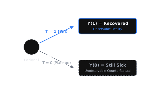
Imagine a patient with a headache. You give them a pill (the treatment, $T=1$), and an hour later, their headache is gone (the outcome, $Y=1$). Did the pill cure the headache?

This missing-data problem is the central dilemma of causal inference.

How It Actually Works

The framework rests on formalizing the idea of alternate realities. For any unit $i$ (a user, a patient, a city) and a binary treatment $T$ (0 for control, 1 for treated), there exist two potential outcomes:

• $Y_i(1)$: The outcome for unit $i$ if they receive the treatment.
• $Y_i(0)$: The outcome for unit $i$ if they do not receive the treatment.

The true causal effect of the treatment on unit $i$—the Individual Treatment Effect (ITE)—is just the difference between these two parallel universes: $\text{ITE}_i = Y_i(1) - Y_i(0)$

The Fundamental Problem of Causal Inference

The fundamental problem is that we only ever observe one of the potential outcomes. The observed outcome $Y_i$ is determined by the treatment actually assigned: $Y_i = T_i Y_i(1) + (1 - T_i) Y_i(0)$

If $T_i = 1$, we observe $Y_i(1)$. The other potential outcome, $Y_i(0)$, becomes an unobservable counterfactual. Because we can never compute $\text{ITE}_i$ directly for any single individual, causal inference is fundamentally a missing data problem.

Average Treatment Effect (ATE)

Since we cannot measure individual effects, we pivot to estimating average effects across a population. The Average Treatment Effect (ATE) is the expected value of the individual effects: $\text{ATE} = \mathbb{E}[Y(1) - Y(0)]$

By linearity of expectation, this becomes: $\text{ATE} = \mathbb{E}[Y(1)] - \mathbb{E}[Y(0)]$

This looks solvable! We just take the average outcome of the treated group and subtract the average outcome of the control group. However, this naive approach only works if a massive assumption holds.

The Independence Assumption

The naive difference in means is: $\text{Naive ATE} = \mathbb{E}[Y | T=1] - \mathbb{E}[Y | T=0]$

This only equals the true $\text{ATE}$ if the treatment assignment $T$ is independent of the potential outcomes: $(Y(0), Y(1)) \perp \!\!\! \perp T$.

If doctors give the pill only to the sickest patients, then the patients in the $T=1$ group have fundamentally different $Y(0)$ baseline values than the patients in the $T=0$ group. The naive difference will be contaminated by selection bias. The only way to guarantee independence in the real world is to assign the treatment randomly.

Show Me the Code

We can simulate potential outcomes to see why observational comparisons fail and why randomization works.

1import numpy as np2import pandas as pd3
4np.random.seed(42)5n_patients = 10006
7# 1. Generate Potential Outcomes (The God View)8# Baseline health: higher is better9health_baseline = np.random.normal(50, 10, n_patients) 10
11# Y(0): Outcome without the pill (mostly just baseline)12Y_0 = health_baseline + np.random.normal(0, 2, n_patients)13
14# Y(1): Outcome with the pill (pill adds exactly +5 health to everyone)15Y_1 = Y_0 + 5.0  16
17# True ATE is exactly 5.018true_ate = np.mean(Y_1 - Y_0)19print(f"True ATE (Unobservable): {true_ate:.2f}")20
21# --- Scenario A: Observational Data (Biased) ---22# Sick patients (health < 50) are more likely to take the pill23prob_treatment = np.where(health_baseline < 50, 0.8, 0.2)24T_obs = np.random.binomial(1, prob_treatment)25
26# We only observe Y(1) if T=1, else Y(0)27Y_obs = np.where(T_obs == 1, Y_1, Y_0)28
29# Naive comparison30naive_ate_obs = np.mean(Y_obs[T_obs == 1]) - np.mean(Y_obs[T_obs == 0])31print(f"Naive ATE (Observational): {naive_ate_obs:.2f}") # Result: ~ -10.0 (Wrong!)32
33# --- Scenario B: Randomized Experiment ---34# Treatment is assigned completely randomly (coin flip)35T_rand = np.random.binomial(1, 0.5, n_patients)36Y_rand = np.where(T_rand == 1, Y_1, Y_0)37
38# Naive comparison on randomized data39naive_ate_rand = np.mean(Y_rand[T_rand == 1]) - np.mean(Y_rand[T_rand == 0])40print(f"Naive ATE (Randomized): {naive_ate_rand:.2f}") # Result: ~ 5.0 (Correct!)

Watch Out For

The Quick Version

• Potential outcomes are the alternate realities where a unit does or does not receive a treatment.
• The Fundamental Problem of Causal Inference is that we can never observe both potential outcomes for the same unit simultaneously; one is always a counterfactual.
• The Average Treatment Effect (ATE) averages these hypothetical differences across a population.
• You can only estimate the ATE using simple group averages if the treatment assignment is completely independent of the potential outcomes (e.g., via a randomized controlled trial).

What to Read Next

• randomized-experiments — How A/B testing physically enforces the independence assumption.
• causal-graphs — A different, visual framework for causal inference that complements potential outcomes.
• ab-testing-for-ml — How to apply this framework to evaluate machine learning models in production.