Randomized Experiments
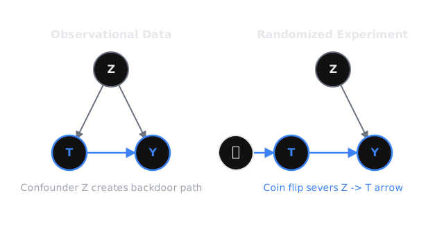
When you flip a coin to decide who gets a treatment, you guarantee that nothing else caused the decision. Randomization severs the link from all confounders, known and unknown.
Why Does This Exist?
In observational data, you can only control for the confounders you measured. If you believe income and age confound the relationship between a marketing email and a purchase, you can add them to your model. But what if "boredom" is also a confounder? What if "propensity to check email at 3 AM" is a confounder? If you didn't measure them, your estimate of the email's effect will be biased, and no amount of math can save it.
Randomized Controlled Trials (RCTs)—or A/B tests—exist to solve the problem of unmeasured confounders. By taking the decision of who gets the treatment completely out of the hands of humans, nature, and algorithms, and handing it to a random number generator, we force the treatment assignment to be completely independent of every other variable in the universe.
Think of It Like This
Imagine trying to figure out if wearing a wetsuit makes you swim faster.
Think of It Like This
If you just look at observational data, you'll see that people wearing wetsuits swim much faster than people in swimsuits. But wait—people in wetsuits are usually professional surfers or triathletes, while people in swimsuits are splashing in a pool. Athleticism is the unmeasured confounder. To find the true effect of the wetsuit, you must take a group of people and flip a coin to decide what they wear. Some triathletes will get swimsuits; some amateurs will get wetsuits. The coin flip breaks the connection between athleticism and the outfit.
How It Actually Works
In the language of Potential Outcomes, we want to estimate the Average Treatment Effect (ATE):
We can only estimate this using the simple difference in observed means () if the treatment is independent of the potential outcomes: . This property is called Exchangeability. It means the treated group and the control group are completely interchangeable; if we swapped their treatments, their average outcomes would swap perfectly.
In the language of Causal Graphs, a confounder creates a backdoor path . When we randomize , we are physically intervening in the system. The equation that normally determines is replaced by a coin flip: . Because now listens only to the coin, the arrow is deleted from the graph. The backdoor path is cut.
The Power of Randomization
Randomization achieves identification—the ability to calculate a causal effect from data—without requiring us to assume we know all the confounders. It handles:
- Measured confounders: Income, age, location.
- Unmeasured confounders: Mood, hidden preferences, systemic bias.
Because the coin flip distributes all these traits equally (on average, given a large enough sample size) between the treatment and control groups, the only remaining difference between the groups is the treatment itself.
Code
Let's simulate a scenario with a massive unobserved confounder, and see how observational regression fails while randomization succeeds perfectly.
import numpy as npimport statsmodels.api as sm
np.random.seed(42)N = 5000
# 'Hidden Motivation' is a massive confounder we cannot measurehidden_motivation = np.random.normal(0, 1, N)
# Treatment: Using an AI study tool (T=1) or not (T=0)# Outcome: Final exam score (Y)
# True causal effect: The tool adds exactly +2 points to the scoretrue_effect = 2.0
# Outcome is driven by baseline (70), the true effect, motivation, and noiseY_0 = 70 + 5 * hidden_motivation + np.random.normal(0, 2, N)Y_1 = Y_0 + true_effect
# --- Observational Data ---# Highly motivated students are much more likely to use the toolprob_T_obs = 1 / (1 + np.exp(-2 * hidden_motivation))T_obs = np.random.binomial(1, prob_T_obs)Y_obs = np.where(T_obs == 1, Y_1, Y_0)
# Naive regression on observational dataX_obs = sm.add_constant(T_obs)model_obs = sm.OLS(Y_obs, X_obs).fit()print(f"Observational Estimate: +{model_obs.params[1]:.2f} points")# -> +10.15 points. WRONG! It credits the tool for the students' motivation.
# --- Randomized Experiment (A/B Test) ---# We force 50% of students to use the tool, 50% to not, completely randomlyT_rand = np.random.binomial(1, 0.5, N)Y_rand = np.where(T_rand == 1, Y_1, Y_0)
# Naive regression on randomized dataX_rand = sm.add_constant(T_rand)model_rand = sm.OLS(Y_rand, X_rand).fit()print(f"Randomized Estimate: +{model_rand.params[1]:.2f} points")# -> +2.07 points. CORRECT! Randomization severed the link to motivation.Watch Out For
Small sample sizes.
Randomization only guarantees balance in expectation. If you flip a coin 10 times, you might get 8 heads. If your experiment only has 20 participants, the treatment group might accidentally end up much older or wealthier than the control group, bringing confounding right back. Randomization requires large to wash out the variance.
Non-compliance.
Just because you randomly assign someone a treatment doesn't mean they actually take it. If users in the treatment group refuse to use the new feature, your estimate of the feature's effect will be diluted. You must distinguish between the Intention-to-Treat (ITT) effect and the actual causal effect (which requires Instrumental Variables to calculate).
The Quick Version
- Observational causal inference requires you to measure and control for every single confounder. This is usually impossible.
- Randomization solves this by breaking the causal arrow from the confounder to the treatment assignment.
- By assigning treatment via a coin flip, you ensure the treatment and control groups are exchangeable, meaning any difference in their outcomes must be caused exclusively by the treatment.
- In causal graph terms, randomization is a structural intervention that deletes all incoming arrows to the treatment node.