Core ML

Recommendation Evaluation

You can't use standard ML metrics like Accuracy or RMSE to judge a search engine. We need metrics that care about the exact position of the correct answer, and metrics that prove we aren't just recommending the same 10 popular things to everyone.

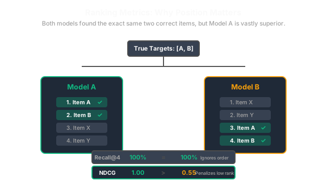
Standard metrics only care IF you got it right. Ranking metrics like NDCG care heavily about WHERE you got it right.

Why Does This Exist?

In traditional machine learning, evaluation is easy. If a model predicts a house costs $400k, and it actually costs$ 410k, the error is $10k.

Recommender systems don't work like this. They output a ranked list of 10 items. If the user clicks the item in Slot 1, that is a massive success. If the user clicks the item in Slot 10, that is technically a success, but it's a very poor user experience. They had to scroll past 9 bad items to find it.

To evaluate a Recommender System offline (before deploying it to A/B testing), we have to use specialized Ranking Metrics that heavily penalize the model for burying the good stuff at the bottom of the list.

Think of It Like This

Imagine asking two librarians to find a specific book.

Librarian A brings you 1 book. It is the exact book you wanted. Librarian B brings you a stack of 100 books. The book you wanted is at the very bottom of the stack.

According to a standard ML metric like "Accuracy" or "Recall", both librarians scored 100%. They both successfully found the book. But according to a Ranking Metric like NDCG, Librarian A scores 100%, and Librarian B scores 2% because they made you dig through 99 irrelevant things first.

The Top 3 Metrics

1. Recall@K (and Precision@K)

The simplest ranking metric. You only look at the Top K items (usually K=10).

Recall@10: Out of all the items the user actually wanted, what percentage were in our Top 10?
Precision@10: Out of the 10 items we recommended, what percentage did the user actually want?
The Problem: It doesn't care about order. Putting the right answer in Slot 1 gives the exact same score as putting it in Slot 10.

2. MRR (Mean Reciprocal Rank)

MRR cares about order, but it assumes the user only wants one single thing (like a Google Search). It looks at the position (the rank) of the first correct item, and calculates $\frac{1}{\text{Rank}}$ .

Correct item is at Rank 1: Score = $1/1 = 1.0$
Correct item is at Rank 2: Score = $1/2 = 0.5$
Correct item is at Rank 10: Score = $1/10 = 0.1$
The Problem: It stops counting after the first success. If you are recommending 10 movies for a weekend, the user might want multiple movies.

3. NDCG (Normalized Discounted Cumulative Gain)

The undisputed king of recommender metrics. It solves all the problems above.

Gain: It handles varying levels of relevance. A movie the user watched for 2 hours gives a higher "Gain" than a movie they watched for 5 minutes.
Discounted: It divides the Gain by the logarithm of the Rank. This heavily penalizes the model for putting highly relevant items at the bottom of the list.
Normalized: It compares the model's list against the mathematically perfect list, outputting a final score between 0.0 (terrible) and 1.0 (perfect).

Non-Accuracy Metrics (The Secret Sauce)

In the real world, a model with perfect NDCG will often fail in A/B testing because it is too boring. A good recommender system must balance accuracy with discovery.

Catalog Coverage: What percentage of your total catalog was recommended to at least one user today? If you have 10,000 items but you only ever recommend the same 50 blockbusters, your Coverage is 0.5%. You are wasting your catalog.
Serendipity / Novelty: How often do you recommend items that the user likes, but that they never would have found on their own? Recommending milk to someone buying cereal has high accuracy but zero novelty.
Diversity: Are all 10 items in the carousel identical? Recommending 10 different Batman comics has high accuracy, but terrible diversity.

Show Me the Code

Evaluating Ranking metrics requires grouping your test data by user/query before calculating the score.

1from sklearn.metrics import ndcg_score2import numpy as np3
4# A single user is shown 5 movies.5# The 'True Relevance' is how much they actually liked it (e.g. 0 to 3 stars)6true_relevance = np.asarray([[3, 2, 0, 0, 1]])7
8# Model A predicts perfect scores. It puts the 3-star movie first.9model_A_scores = np.asarray([[0.9, 0.8, 0.1, 0.2, 0.5]])10print(f"Model A NDCG: {ndcg_score(true_relevance, model_A_scores):.2f}")11# Output: 1.0012
13# Model B predicts the exact same scores, but reversed. 14# It puts the 3-star movie at the very bottom (Rank 5).15model_B_scores = np.asarray([[0.1, 0.2, 0.8, 0.9, 0.5]])16print(f"Model B NDCG: {ndcg_score(true_relevance, model_B_scores):.2f}")17# Output: 0.6118
19# Notice that the Discount (the D in NDCG) heavily penalized Model B 20# for burying the good movie at the bottom of the list.

Watch Out For

Offline metrics are liars. NDCG is calculated on historical, offline data. It can only evaluate items the user actually interacted with in the past. If your new model recommends an obscure indie movie that the user would love, NDCG will score it as a failure (Relevance=0) simply because the user hasn't seen it yet. You must use A/B Testing or Contextual Bandits to prove a model actually works in the real world.

The Quick Version

Standard ML metrics like Accuracy ignore the position of the item in the list.
Recall@K measures if the good items were in the Top K, but still ignores order.
MRR heavily rewards putting the first correct item at the very top of the list.
NDCG is the industry standard. It evaluates the entire list, rewarding highly relevant items, and logarithmically penalizing items that are buried too deep.
Accuracy isn't everything. You must also monitor Coverage and Diversity to ensure you aren't just blindly recommending popular items.

Related concepts

Contextual Bandits