Core ML

Sliding Window Attention

Each token only attends to the nearest W tokens around it instead of every token in the sequence, so attention cost scales linearly with sequence length rather than quadratically.

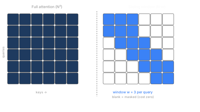
Why Does This Exist?

Full self-attention lets every token attend to every other token. That's exactly the property that makes it powerful — a token at position 8,000 can directly use information from position 1 — but it's also what gives it quadratic cost. Double the sequence length and you quadruple the work, as attention complexity makes precise.

The observation motivating sliding window attention is that for many tasks, most of the useful context is local. In language modelling, a word strongly depends on the words nearby; in code, the relevant variable declaration is usually within a few hundred tokens. Long-range dependencies matter too, but they tend to be sparse — a few specific tokens are relevant, not the entire prefix.

Sliding window attention captures the local part cheaply: each query attends only to the W nearest tokens. Cost falls from $O(N^2)$ to $O(N \cdot W)$ . Longformer (2020) demonstrated that the local window alone, combined with a few global tokens, was enough to handle document-length tasks that broke standard attention. Mistral 7B uses a window of 4,096 tokens on top of rotary embeddings, making a 32K context tractable on a single GPU.

Think of It Like This

Reading a book through a magnifying glass

You're summarising a 1,000-page book, but your magnifying glass only reveals a window of 20 pages at a time. You slide the window forward, page by page, taking notes as you go. Each note captures what the current window says — but no note looks back at what the glass couldn't reach.

That's sliding window attention. The glass is the window W; the notes are the representations built at each position; the "looking back at what the glass couldn't reach" is what global tokens (or later layers) handle when you need long-range information.

How It Actually Works

The restricted score matrix

Standard attention computes an $N \times N$ score matrix and fills every cell. Sliding window attention computes only the cells within a band of width $W$ around the diagonal — specifically, for query at position $i$ , only keys at positions $\max(0, i - W/2)$ to $\min(N-1, i + W/2)$ enter the score computation.

In causal (autoregressive) models, the window is one-sided: query $i$ attends to positions $\max(0, i - W)$ through $i$ . Cost: $O(N \cdot W)$ per layer, versus $O(N^2)$ for full attention.

Receptive field through depth

A single sliding-window layer has limited global reach. But stacking $L$ layers with window $W$ gives an effective receptive field of $L \cdot W/2$ tokens, growing linearly with depth. A 32-layer model with window 4,096 can propagate information from up to 65,536 tokens away through the stack — covering a 65K context without any single layer attending that far.

This is how Mistral 7B handles 32K contexts with 4,096-token windows: the lower layers handle local structure; the upper layers, receiving representations built by lower layers, effectively have long-range awareness through composition.

Combined with global tokens

Pure local windowing loses genuinely long-range dependencies that don't propagate through enough layers in time. Longformer adds a small set of "global" tokens (CLS, question tokens in QA) that attend to every position and every position attends back to them — an $O(N \cdot g)$ cost for $g$ global tokens, typically $g \ll N$ .

Show Me the Code

Measuring the score computation budget for full vs. sliding window attention across a range of sequence lengths.

1import numpy as np2
3W = 4096  # Mistral's window size4
5def full_attention_cells(n: int) -> int:6    return n * n7
8def sliding_window_cells(n: int, w: int) -> int:9    # For causal window: each query attends to min(w, i+1) positions10    return sum(min(w, i + 1) for i in range(n))11
12for n in (4_096, 8_192, 32_768):13    full = full_attention_cells(n)14    local = sliding_window_cells(n, W)15    print(f"n={n:>6}  full={full:>12,}  window={local:>10,}  ratio={full/local:.1f}×")16# n=  4096  full=  16,777,216  window= 8,390,656  ratio=2.0×17# n=  8192  full=  67,108,864  window=20,967,424  ratio=3.2×18# n= 32768  full= 1,073,741,824  window=115,343,360  ratio=9.3×

At 32K tokens, sliding window with W=4,096 requires only about 11% of the score cells that full attention needs. The advantage grows with N, which is exactly when you need it most.

Watch Out For

Assuming local windows handle all long-range dependencies

Sliding window attention cannot directly connect tokens separated by more than W positions in a single layer. For tasks where a token at the very end of a long document genuinely needs a fact from the very beginning — and that fact doesn't propagate through intermediate representations naturally — a pure local window will miss it. Global tokens, hierarchical attention, or a retrieval step are needed to bridge that gap. The window is not a shortcut that costs nothing; it's a trade-off that matches the locality assumption of many but not all tasks.

Expecting linear memory in the KV cache

The score computation per layer is $O(N \cdot W)$ , but the KV cache at autoregressive inference still stores the keys and values of all previous tokens — up to N of them — not just the window. The window limits which of those cached entries are used at each step, but they still have to be stored. Actual KV cache memory savings require eviction strategies, like those in attention sinks.

The Quick Version

Each query attends only to the W nearest tokens; cells outside that band are masked and cost nothing.
Compute drops from $O(N^2)$ to $O(N \cdot W)$ per layer — a factor-of- $N/W$ reduction.
Global reach accumulates through depth: $L$ layers of window $W$ reach $L \cdot W/2$ tokens away.
The KV cache at inference still grows with N unless explicit eviction is added.
Mistral 7B uses a 4,096-token window to serve a 32K context on a single GPU.