Core ML

Survival Analysis

Standard classification answers 'Will this user churn?'. Survival Analysis answers a much more useful question: 'How long until this user churns?'

A survival curve shows the probability of a user 'surviving' (not churning) over time. As time passes, the probability drops as users slowly leave the platform.

Why Does This Exist?

If you are trying to predict customer churn, you might naturally build a binary classification model (Propensity to Churn). You label users who left as 1 and users who stayed as 0. But there is a massive logical flaw in this approach: everyone eventually churns. If you look far enough into the future, the probability of churn for every user is exactly 100%.

Binary classification forces you to pick an arbitrary time horizon: "Will they churn in the next 30 days?". But what if they churn on day 31? What about day 400? Classification throws away all the nuance of time.

Survival Analysis (also known as Time-to-Event analysis) solves this. Originally developed by medical statisticians to predict patient lifespans, it allows data scientists to model the continuous probability of an event happening across the entire timeline of a user's lifecycle.

Think of It Like This

Imagine you are managing a fleet of rental cars. You want to know when the engine in Car A will break down. If you use Binary Classification, you ask: "Will it break down this week?" The answer is "No." If you use Regression to predict the exact days until failure, you run into a problem: Car B hasn't broken down yet, so what number do you put as its label?

Survival Analysis allows you to say: "Car A has a 99% chance of surviving Month 1, an 80% chance of surviving Month 6, and a 10% chance of surviving Month 12." You get a complete curve of probability over time.

How It Actually Works

Survival Analysis revolves around two core concepts: Censoring and the Survival Function.

1. Censoring (The Missing Data Problem)

In standard ML, every row needs a label. In time-to-event data, what do you do with a user who subscribed yesterday? They haven't churned yet. Do you label them as "Did not churn"? That's inaccurate; they might churn tomorrow. Do you delete their row? That introduces massive survivorship bias.

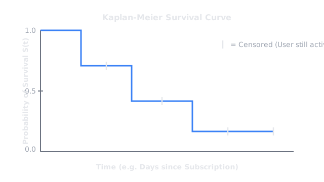
This is called Right-Censoring. We know the user survived at least until today, but we don't know what happens after. Survival algorithms are mathematically designed to learn from censored data without requiring a final outcome.

2. The Survival Function $S(t)$

Instead of a single probability, the output of a survival model is a curve $S(t)$ . It represents the probability that the event has not occurred by time $t$ . At $t=0$ , $S(t) = 1.0$ . As $t \rightarrow \infty$ , $S(t) \rightarrow 0$ .

Core Algorithms

Kaplan-Meier Estimator: A simple, non-parametric way to draw a survival curve for an entire population or a specific segment (e.g., comparing the survival curve of free users vs. paid users).
Cox Proportional Hazards: A regression model that figures out how different features (age, income) multiply the underlying risk (hazard) of the event happening.
Machine Learning Survival Models: Algorithms like Random Survival Forests or XGBoost Survival that can handle non-linear relationships and high-dimensional tabular data.

Show Me the Code

You can use the lifelines library in Python to quickly build and plot survival models.

1import pandas as pd2from lifelines import KaplanMeierFitter, CoxPHFitter3import matplotlib.pyplot as plt4
5# Data requires two columns:6# T: Duration (Time observed)7# E: Event observed (1 if churned, 0 if censored/still active)8
9# 1. Kaplan-Meier (Population Level)10kmf = KaplanMeierFitter()11kmf.fit(durations=df['T'], event_observed=df['E'])12kmf.plot_survival_function()13plt.title("Overall Customer Survival Curve")14plt.show()15
16# 2. Cox Proportional Hazards (Feature Level)17# We want to know how 'Age' and 'Monthly_Spend' affect the time to churn18cph = CoxPHFitter()19cph.fit(df, duration_col='T', event_col='E')20cph.print_summary()21
22# 3. Predict the survival curve for a specific new user23new_user = pd.DataFrame({'Age': [30], 'Monthly_Spend': [50.0]})24survival_curve = cph.predict_survival_function(new_user)25print(survival_curve.head())26# Output is a Pandas Series where the index is Time (t) 27# and the values are the Probability of Survival at that time.

Watch Out For

Informative Censoring. Standard survival models assume that censoring is random (e.g., the data simply ends today). But if users are dropping out of your dataset for a reason related to the event (e.g., users cancel their subscription because they are moving to a competitor before they officially "churn"), your model will be biased. You must understand why data is censored.

The Quick Version

Standard classification models force you to pick an arbitrary time window for events like churn or failure.
Survival Analysis predicts the probability of an event happening over a continuous timeline.
It is the only statistically valid way to handle Right-Censored Data (users who haven't experienced the event yet).
The output is a Survival Curve $S(t)$ showing the probability of survival across time.