Time Series Decomposition
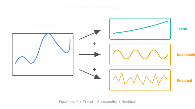
The mathematical process of breaking a time series down into three distinct components: the overall trend, the repeating seasonal pattern, and the random noise.
Why Does This Exist?
When you look at a graph of monthly airline passengers over a decade, it looks like a jagged, messy line heading up and to the right.
If you try to forecast that raw line directly, models often fail because they get confused by the combination of long-term growth and short-term spikes (like summer holidays).
Time Series Decomposition solves this by splitting the raw data into three mathematically distinct layers. It is almost always the very first step a data scientist takes when analyzing time-stamped data, because forecasting the three layers independently is drastically easier than forecasting the raw signal.
Think of It Like This
Think of It Like This
Imagine you are listening to a symphony orchestra play a complex piece of music.
If you record the raw audio, it's just one massive, complicated sound wave.
Decomposition is like running that audio through a mixing board to isolate the individual instruments. You isolate the steady, slow beat of the cello (the Trend). You isolate the fast, repeating melody of the violins (the Seasonality). And whatever background static is left over is the Residual noise. By looking at the instruments separately, you understand exactly how the song is constructed.
How It Actually Works
The classical approach assumes that any observation at time is simply a combination of three unobserved components.
Depending on how the variance of the data behaves, we use either an Additive or Multiplicative model.
1. The Additive Model
Use this when the seasonal swings stay roughly the same size over time, regardless of the trend.
2. The Multiplicative Model
Use this when the seasonal swings get larger as the trend grows (e.g., a company's holiday sales spike gets bigger every year as the company grows).
Extracting the Components
Modern libraries use STL (Seasonal and Trend decomposition using Loess). It works in a loop:
- It applies a smoothing function (moving average or Loess) to the raw data to extract the slow-moving Trend.
- It subtracts the Trend from the raw data (leaving only seasonality + noise).
- It averages the data across seasonal periods (e.g., averaging all Januaries together) to extract the pure Seasonality.
- It subtracts the Seasonality. Whatever is left over is the unpredictable Residual.
Code
In Python, the statsmodels library handles decomposition out of the box.
import pandas as pdimport matplotlib.pyplot as pltfrom statsmodels.tsa.seasonal import seasonal_decompose
# Create dummy monthly data (Trend + Seasonality + Noise)dates = pd.date_range(start='2020-01-01', periods=24, freq='M')data = [10, 12, 15, 20, 25, 30, 28, 22, 18, 15, 12, 11, 15, 18, 20, 25, 30, 35, 33, 27, 23, 20, 17, 16]
ts = pd.Series(data, index=dates)
# Perform additive decomposition with a period of 12 (months)result = seasonal_decompose(ts, model='additive', period=12)
# Plot the separated componentsresult.plot()plt.show()
# Access the underlying numbersprint("Trend:\n", result.trend.dropna().head())print("\nSeasonality:\n", result.seasonal.dropna().head())print("\nResiduals:\n", result.resid.dropna().head())Watch Out For
Residuals are the reality check.
If you run a decomposition and the "Residual" component still has a clear repeating pattern in it, your decomposition failed. It means there is a seasonal pattern (perhaps a weekly cycle hiding inside a monthly cycle) that you haven't extracted yet. Residuals should look completely random (white noise).
Multiple Seasonalities.
Standard decomposition assumes a single seasonal period (e.g., just yearly). High-frequency data (like server CPU usage recorded every minute) often has multiple seasonalities (daily dips at night, and weekly dips on weekends). You must use advanced algorithms like MSTL (Multiple STL) to extract overlapping seasonal patterns.
The Quick Version
- Time series decomposition breaks a single messy metric into three clean components.
- Trend: The long-term direction of the data.
- Seasonality: The short-term, strictly repeating pattern.
- Residual: The unpredictable, random noise left over.
- It is fundamentally easier to build separate ML models to forecast the trend and seasonality individually than to forecast the raw data.