Core ML

Universal Approximation

A wide-enough single hidden layer can get within any accuracy you name of any continuous function on a bounded domain — but the theorem only proves such weights exist, never that gradient descent can find them or that the required width is affordable.

A single hidden layer fitting the same wiggly target function at four widths: two units barely traces the shape, fifty units overlays the target almost exactly — width, not depth, is what the theorem promises here

Why Does This Exist?

"A neural network can approximate any function" gets repeated often enough that it starts to sound like a guarantee you can build on — proof that if a relationship between inputs and outputs exists at all, some network somewhere can learn it. That statement is close to true, and it's also one of the most over-claimed sentences about neural networks in casual conversation, because what it actually promises is narrower, and less immediately useful, than it sounds.

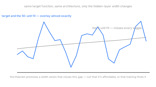
Here's what a single hidden layer, fitting the wiggly two-frequency function $\sin(3x) + 0.5\cos(7x)$ , actually does as it gets wider: with 2 hidden units the fit barely traces the shape at all, mean squared error over 0.6. Widen it to 10 units and the error drops to 0.15 — closer, but visibly wrong in places. At 50 units the error rounds to zero — a near-perfect trace. Nobody changed the depth, the activation function, or the training procedure between those runs. Width alone closed the gap, and that's exactly the phenomenon the universal approximation theorem formalizes — and exactly where its promise stops.

Think of It Like This

Tracing a curve with an ever-larger box of french curves

A french curve is a rigid, curved plastic template draftsmen use to trace smooth lines by hand — one template traces one specific shape of curve well and everything else poorly. Hand someone exactly two french curves and ask them to trace an intricate, wiggly line on a blueprint, and they'll get the rough shape but miss every fine wiggle the two templates don't match.

Now hand them a box of fifty french curves, every one a slightly different shape, and let them piece the line together from short segments, each traced with whichever template fits that stretch best. With enough templates in the box, any line — however wiggly — can be traced to any precision asked for, one small segment at a time.

That's the promise being made: with enough templates, any curve can be assembled. It says nothing about whether the draftsman can quickly find the right fifty templates from a box of a million candidates, or whether a smaller, cleverer box — arranged in stages instead of piled in one heap — might trace the same line with far fewer templates.

How It Actually Works

What the theorem actually states

Proved for sigmoid units by Cybenko in 1989 and generalized to a broad class of activations since: for any continuous function $f$ on a compact (closed and bounded) domain, and any error tolerance $\varepsilon > 0$ you name in advance, there exists a single-hidden-layer network — some width $m$ , some weights — whose output stays within $\varepsilon$ of $f$ everywhere on that domain. Every qualifier in that sentence is load-bearing: compact domain (the guarantee doesn't extend to unbounded inputs), non-polynomial activation (a polynomial activation provably can't achieve this, no matter the width), and existence — the theorem proves such weights are out there, not that any particular training procedure finds them.

Existence is not learnability

That last qualifier is the one people quietly drop, and it's the one that matters most in practice. The theorem is a pure existence proof: it establishes that suitable weights exist somewhere in an astronomically large space of possible weight configurations. It says nothing about whether gradient descent, starting from a random initialization, can actually navigate to that configuration in any reasonable number of steps. A function can be exactly representable by some network and still be practically unlearnable by the training procedure anyone would actually run.

The other missing number: how wide is "wide enough"

The theorem also says nothing about $m$ , the required width, beyond the fact that some finite value works. For some target functions, $m$ stays small and manageable. For others — including some fairly natural functions — the width needed to hit a given error tolerance with a single hidden layer grows so large that the network becomes computationally unaffordable, even though the theorem still guarantees a solution exists somewhere in principle. That gap is exactly why depth still matters: a target built from staged, composable sub-patterns often needs exponentially fewer parameters when represented as several narrower layers stacked in sequence, rather than flattened into one very wide layer forced to represent every stage's combination directly.

Show Me the Code

The same target function, one hidden layer, four widths — measuring how test error actually falls as $m$ grows, rather than asserting that it does.

1import numpy as np2
3
4def target(x: np.ndarray) -> np.ndarray:5    return np.sin(3 * x) + 0.5 * np.cos(7 * x)6
7
8def fit_one_hidden_layer(x_train, y_train, x_test, width, seed=0):9    rng = np.random.default_rng(seed)10    w1, b1 = rng.normal(scale=3.0, size=(1, width)), rng.uniform(-3, 3, size=width)11    h_train = 1 / (1 + np.exp(-(x_train[:, None] @ w1 + b1)))  # sigmoid hidden layer12    h_test = 1 / (1 + np.exp(-(x_test[:, None] @ w1 + b1)))13    w2, *_ = np.linalg.lstsq(h_train, y_train, rcond=None)  # fit only the output layer14    return h_test @ w215
16
17x = np.linspace(-3, 3, 400)18x_test = np.linspace(-3, 3, 200)19y, y_test = target(x), target(x_test)20
21for width in (2, 10, 50):22    mse = np.mean((fit_one_hidden_layer(x, y, x_test, width) - y_test) ** 2)23    print(f"width {width:3d}: test MSE = {mse:.4f}")24# -> width   2: test MSE = 0.602325# -> width  10: test MSE = 0.147026# -> width  50: test MSE = 0.0000

Nothing changed between the three runs except $m$ , the hidden layer's width. Error falls from 0.60 to essentially zero purely from adding units — exactly the theorem's promise, made numerically concrete rather than asserted.

Watch Out For

Citing the theorem as a reason not to think about architecture

"A network can approximate anything" gets used to justify skipping architecture design entirely — just make one layer wide enough and stop worrying about depth, inductive bias, or structure. The theorem can't be violated, which also means it can't help decide anything: it doesn't say the required width is affordable, and it doesn't say gradient descent from a chosen initialization will find the right weights within any realistic training budget. Reading flat, plateaued training curves as "the theorem promised this would work" rather than "capacity is available but the optimizer or the width isn't finding it" is the exact misreading this page exists to head off.

Widening a hidden layer instead of adding a second one

A wide single layer stuck at a disappointing error rate sometimes gets doubled or quadrupled in width, on the theory that "wide enough" just hasn't been reached yet — matching the theorem's letter while missing what it actually costs. For functions that are naturally staged or hierarchical, a second hidden layer of similar total size very often reaches lower error than doubling the first layer's width, because depth represents staged composition directly instead of forcing one flat layer to approximate every stage's interaction on its own.

The Quick Version

The theorem guarantees a wide-enough single hidden layer can approximate any continuous function on a bounded domain to any accuracy named in advance.
Every qualifier matters: a compact domain, a non-polynomial activation, and existence rather than a recipe for finding the weights.
It's an existence proof, not a learnability guarantee — nothing here says gradient descent can find those weights in practice.
"Wide enough" is unspecified and can be exponentially large for some functions, which is the real, practical reason depth still matters.
Measured directly, error can fall from 0.6 to near zero purely from adding width — the theorem's promise made concrete, not just asserted.