Core ML

Vanilla RNN

Reuse the same small network at every time step, and let a hidden state carry forward whatever happened earlier so order in the sequence actually matters.

Unrolled across three time steps, an RNN is the same cell and the same weights reused at every step, with the hidden state carrying context from one step into the next

Why Does This Exist?

Feed a sentence into a multi-layer perceptron one word at a time and something's missing immediately: the network has no memory. Show it "bank" after "river" and it processes exactly the same as "bank" after "money" — nothing carries over. A fixed-size feedforward net also wants a fixed-size input, and sentences don't come in one length.

The actual problem is order. "Dog bites man" and "man bites dog" share every word and mean opposite things. A network that treats a sentence as an unordered bag of words can't tell them apart, and plenty of real tasks hinge on exactly that difference.

A recurrent neural network fixes both problems with one idea: process the sequence one element at a time, and keep a running summary — the hidden state — that gets updated at every step and carried into the next one. The network doesn't need to know the sequence length in advance, because it isn't looking at the whole thing at once. It's looking at one token and one summary of everything before it.

Think of It Like This

Reading a novel one page at a time, with a running mental summary

You don't hold every word of a 300-page novel in your head simultaneously. You read page 40, update your understanding of the plot, then read page 41 with that updated understanding already in place — you don't re-read pages 1 through 40 to catch up.

That running mental summary is the hidden state. It doesn't store every word you've read; it's a compressed sketch of what mattered so far. Read a plot twist on page 41 and your summary updates. Forget a minor character's name from page 3, and it might just be gone — the summary only has so much room, and that's exactly the limitation that motivates everything that comes after this page.

How It Actually Works

One cell, reused every step

At each time step $t$ , the cell takes two inputs — the current element $x_t$ and the previous hidden state $h_{t-1}$ — and produces a new hidden state:

h_t = \tanh(W_{xh} x_t + W_{hh} h_{t-1} + b)

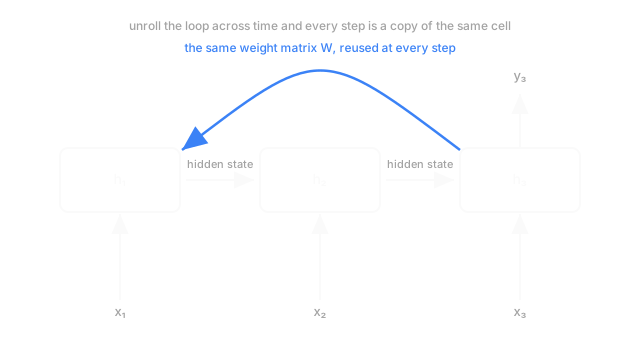
$W_{xh}$ maps the input into the hidden space, $W_{hh}$ maps the previous hidden state into it, $b$ is a bias, and $\tanh$ squashes the result into $(-1, 1)$ . The critical detail, visible in the diagram above: $W_{xh}$ , $W_{hh}$ , and $b$ are the same three objects at every single time step. There's one cell, applied $T$ times for a sequence of length $T$ — not $T$ separate cells. That's what "recurrent" means, and it's also why an RNN handles any sequence length: the same small set of weights just gets reused however many times the sequence requires.

An output, when you need one at every step (tagging each word's part of speech, say), comes from a separate readout $y_t = W_{hy} h_t$ , applied to the hidden state at each position.

Training through time

Because the same weights appear at every step, training an RNN means running backpropagation through the unrolled graph — treating $T$ time steps as $T$ layers that share parameters. This variant is called backpropagation through time (BPTT): the gradient flows backward through every hidden state, and gradients for the shared weights accumulate across every step where those weights were used. $W_{hh}$ contributed to $h_1$ , $h_2$ , and every state after, so a 200-token sequence means 200 terms feeding one weight's update — both the source of an RNN's power and of its most famous training difficulty.

Where it runs into trouble

Chain the recurrence back through many steps and $\partial h_t / \partial h_1$ becomes a product of roughly $t - 1$ Jacobians of $W_{hh}$ passed through $\tanh$ . Multiply many such numbers together and the result shrinks toward zero or grows without bound — vanishing or exploding gradients. In practice, vanilla RNNs reliably lose the signal from more than about 10 to 20 steps back: the running summary has finite room, and a plain RNN's update can't reliably hold onto anything that happened long ago.

Show Me the Code

A single RNN cell, run for three steps by hand, so the "same weights every step" claim is visible in the loop rather than asserted.

1import numpy as np2
3
4def rnn_step(5    x_t: np.ndarray, h_prev: np.ndarray, w_xh: np.ndarray, w_hh: np.ndarray, b: np.ndarray6) -> np.ndarray:7    return np.tanh(w_xh @ x_t + w_hh @ h_prev + b)  # one cell, called again each step8
9
10rng = np.random.default_rng(0)11w_xh, w_hh, b = rng.normal(scale=0.5, size=(4, 3)), rng.normal(scale=0.5, size=(4, 4)), np.zeros(4)12
13h = np.zeros(4)  # h_0, before the sequence starts14for t, x_t in enumerate([np.array([1.0, 0.0, 0.0]), np.array([0.0, 1.0, 0.0]), np.array([0.0, 0.0, 1.0])]):15    h = rnn_step(x_t, h, w_xh, w_hh, b)  # w_xh, w_hh, b never change across the loop16    print(f"h_{t + 1} = {np.round(h, 3)}")17# -> h_1 = [ 0.36  -0.245  0.325 -0.031]18# -> h_2 = [ 0.302 -0.328  0.6   -0.328]19# -> h_3 = [ 0.229 -0.325  0.437 -0.505]

Three calls to the same rnn_step, with w_xh, w_hh, and b untouched throughout — that's the entire architecture. Everything else in this band is a variation on what happens inside that one function.

Watch Out For

Blaming the data when gradients vanish

A vanilla RNN trained on long sequences plateaus early, and the instinct is to add more data, more epochs, or a bigger hidden size. None of that fixes vanishing gradients, because the problem isn't capacity — it's that the gradient for anything more than a few steps back is numerically close to zero before it ever reaches the weights that would need it. More training just repeats the same underpowered update.

The tell: the network learns short-range patterns fine (next-word patterns within a few tokens) but never picks up anything that depends on context from far earlier in the sequence, no matter how long you train. That's an architecture problem, not a data problem — it's what LSTMs and GRUs exist to fix.

Truncating BPTT and forgetting you did

Backpropagating through a 10,000-step sequence is expensive, so implementations often cut the backward pass off after some fixed window — truncated BPTT — while still running the forward pass across the whole sequence. That's a reasonable trade, but it silently caps how far back credit can ever be assigned, regardless of what the forward hidden state might in principle carry. Know the truncation window you're training with, and don't expect the model to learn dependencies longer than it.

The Quick Version

An RNN applies one cell, with one set of weights, repeatedly across a sequence — not a separate cell per position.
The hidden state is a fixed-size running summary, updated at every step from the current input and the previous hidden state.
Training uses backpropagation through time: unroll the recurrence into steps, then backpropagate as if through a deep network with shared weights.
Gradients through many steps are a long product of Jacobians, which vanishes or explodes — vanilla RNNs reliably struggle past 10 to 20 steps.
Any sequence length works with the same weights, which is the whole point of "recurrent."