Data Concepts

Audio Data Preparation

One second of speech at 16kHz is 16,000 numbers. Most audio models want a time-frequency picture instead, and every parameter in that chain is a decision.

A waveform becomes a mel spectrogram, with one 25ms window and its 10ms hop drawn on the wave so the overlap is visible, and that single window producing exactly one column of the picture

Why Does This Exist?

One second of speech at 16kHz is 16,000 numbers. Thirty seconds is 480,000, in a flat 1-D array where the structure you care about lives in how fast the values wiggle rather than in the values.

You can hand that array to a network, and a few architectures do. Most turn the waveform into a picture first: time along one axis, frequency up the other, brightness for energy. That's a mel spectrogram, and once you have one you can point an image model at it.

The chain that builds it has about eight parameters, and every one is a modelling decision, not a setting. Change the window length and you change what the model can resolve. Change the sample rate and you change the pitch of everything it hears.

Think of It Like This

Writing down music by ear

You're transcribing a recording, and you get to choose how long you listen before writing anything down.

Listen for two whole seconds and you can name every note in the chord. But you've no idea when it changed, and if it changed twice you heard a blur.

Listen in flashes of a twentieth of a second and the timing is exact, but you can't tell what the notes were. There wasn't enough sound to carry a pitch.

No setting gives you both. Speech work settles around 25 milliseconds because that's about the shortest listen that still resolves the pitches in a vowel.

How It Actually Works

Sample rate, and the failure that starts here

16kHz is the speech standard, 44.1kHz the audio one. Resampling down is lossy: the Nyquist limit is half the sample rate, so 16kHz discards everything above 8kHz. Fine for speech, less fine for music.

The failure is arithmetic. A model trained at 16kHz, handed a 44.1kHz array nobody resampled, reads 44,100 samples as 2.76 seconds instead of one. Everything is pitched down and stretched, the array is valid, and nothing errors.

Amplitude, and what clipping destroys

int16 samples run −32,768 to 32,767, so dividing by 32,768 gives floats in −1 to 1.

Then a level choice. Peak normalisation scales until the loudest sample hits 1, which one stray click can dominate. Loudness normalisation targets perceived level across the clip, better when sources differ. Don't let either clip: a clipped sample is flattened at the ceiling, the peak is gone for good, and the flat top adds harmonics the recording never had.

Mono, then framing

Downmix to mono by averaging the channels, or a mono model reads alternate samples from alternate ears.

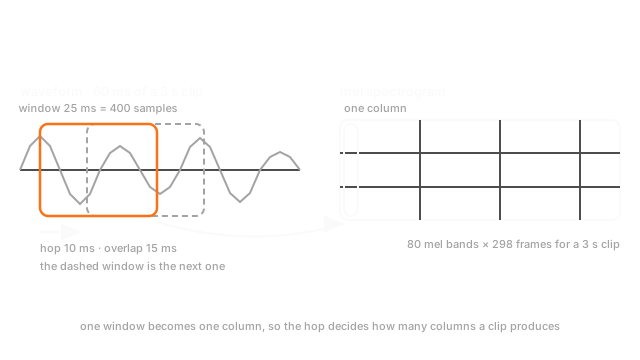
Framing is where the trade lives. Window length sets frequency resolution, hop length sets time resolution, and they pull against each other. A 25ms window at 16kHz is 400 samples with bins about 40Hz apart; a 10ms hop is 160 samples, so 100 frames a second.

Hard window edges imply a discontinuity the signal never had, and the transform reports it as energy smeared across frequencies that weren't there. Hann tapers to zero at both ends.

From spectrogram to mel

The short-time Fourier transform runs on each window and returns complex numbers. Take the magnitude, stack the columns, and you have a spectrogram: 512 points at 16kHz gives 257 bins, 31.25Hz apart, linearly.

Linear spacing is wrong for hearing. 100 to 200Hz is an octave and obvious, 7,000 to 7,100Hz is inaudible. The mel filterbank sums linear bins into fewer bands, narrow at the bottom and wide at the top, so 257 bins become 80 of roughly equal perceptual weight.

Then a logarithm, because magnitudes span orders of magnitude and loudness is perceived logarithmically. That's log-mel, what most audio models eat. MFCCs decorrelate those bands with a cosine transform, which mattered when models assumed independent features and doesn't now.

Silence, length, and the fact that it's a picture

Voice activity detection finds the speech and trims the rest. Decide once, since trimming moves the length distribution and the loudness statistics.

Clips vary in length and batches don't, so pad to the longest with a mask, or cut fixed chunks.

A mel spectrogram is a 2-D array of intensities, so image preparation carries over, augmentation included. SpecAugment masks bands of frequency and time.

Worked example

Three seconds at 16kHz is 48,000 samples, window 400, hop 160.

Each hop after the first window adds a frame while a whole window still fits: 48,000 minus 400, over 160, floored, plus one. So 47,600/160 = 297.5, meaning 297 whole hops and 298 frames, and with 80 mel bands the picture is 80 × 298. Libraries that pad the edges report 301 instead.

The same three seconds at 44.1kHz, sent through unchanged: 132,300 samples gives 825 frames, so the model reads 8.27 seconds, pitched down by 2.76, through a filterbank built for a different range.

Show Me the Code

1import numpy as np2
3SR: int = 16_0004win: int = int(0.025 * SR)                                    # 25ms window5hop: int = int(0.010 * SR)                                    # 10ms hop6clip: np.ndarray = np.sin(2 * np.pi * 440 * np.arange(3 * SR) / SR)7
8
9def frames(n_samples: int, window: int, stride: int) -> int:10    """Windows that fit without padding: the whole hops, plus the first window."""11    return (n_samples - window) // stride + 112
13
14print(clip.shape[0], win, hop)                # -> 48000 400 16015print(frames(clip.shape[0], win, hop))        # -> 29816print((80, frames(clip.shape[0], win, hop)))  # -> (80, 298)17print(frames(3 * 44_100, win, hop))           # -> 82518print(round(44_100 / SR, 3))                  # -> 2.756

The last two lines are the pitfall: the same three seconds, 825 columns instead of 298, pitched down by 2.756.

Watch Out For

A sample rate that differs between training and serving

Your training set was resampled to 16kHz in a job months ago. Serving reads whatever the client uploads: phones send 44.1kHz, browsers 48kHz, a telephony bridge 8kHz.

Nothing errors. Each is a valid float array of a valid shape and the model consumes it happily. What it hears is the recording at the wrong speed: 44.1kHz read as 16kHz is stretched by 2.756 and dropped an octave, so every formant lands in the wrong mel band. An 8kHz clip has nothing above 4kHz, leaving the top of the picture empty.

The symptom is a word error rate worse on some client types than others, which reads as an accent problem long before anyone checks a header.

Resample explicitly on load, in the same function training used, and make the rate part of the data contract.

Normalisation and trimming whose statistics move

Training normalised each clip against its own peak. Serving normalises each batch against the batch peak. Same code path, different scope, so one clip's numbers now depend on which clips arrived with it.

The silence version is quieter. Trimming got added to the training job to save disk and serving never got it, so training clips start on speech while serving clips start with two seconds of room tone. The model has never seen a leading silence that long.

Both are the same mistake as a scaler refitted per batch: the transform is no longer a function of one input.

Fix the scope in code, keep trimming in both places, and ship the transform with the model. See online/offline skew and feature scaling.

The Quick Version

Audio arrives as a long 1-D array, and most models want a 2-D time-frequency picture.
Sample rate first. Resampling down discards everything above half the new rate, and a mismatch at serving pitches and stretches everything, silently.
Divide int16 by 32,768 for floats in −1 to 1, and never let normalisation clip.
Window length buys frequency resolution, hop buys time resolution, and you can't have both. A hard-edged window smears energy that was never there.
The mel filterbank matches how pitch is heard, the log matches loudness, and MFCCs go further than a convolutional net needs.
A mel spectrogram is a picture, so image models and image augmentation apply, SpecAugment included.
Trim and normalise with the same scope on both sides, or the input distribution moves.