Data Concepts

Latent Spaces and Manifold Learning

Real data fills a tiny curved sliver of the space it is stored in. A latent space is the coordinate system on that sliver, and it is where generation works.

Two real points sit on a curved surface, and the straight line between them leaves that surface entirely, which is why interpolating in the input space invents things that are not data

Why Does This Exist?

Here's a claim worth taking literally, because everything on this page and most of generative modelling follows from it. Real data occupies a vanishingly small, curved, low-dimensional subset of the space it's stored in.

Count it. A 100 × 100 greyscale image is 10,000 numbers, each 0 to 255, so there are $256^{10000}$ possible images — a 1 followed by about 24,082 zeros. Now sample one uniformly at random. You get static. Sample every microsecond for the age of the universe and you still get static, every time. You will never hit a face, a cat, or a page of text.

So the set of images that look like anything is unimaginably tiny inside the space that holds it. And it's smooth: rotate a head two degrees and you're still in the set of faces, brighten it slightly and you're still in it. A tiny, smooth, curved subset is what mathematicians call a manifold, and the claim above is the manifold hypothesis.

The intrinsic dimension is how many numbers actually vary. A photo of one person under studio lighting might be described by pose, expression, lighting angle and a handful of other things — maybe 30 numbers, stored as 10,000.

Think of It Like This

A road across a mountain range

You're standing at a village. Another village sits 40km away, and there's a road between them: winding, over a pass, along a valley floor.

Now draw a straight line between the two villages on the map and walk it. Every point on that line is a real place with real coordinates, and most of them are halfway up a cliff. The line is geometrically valid and physically useless.

The road is the manifold. It's one-dimensional — one number, "how far along", locates you exactly — even though it's drawn on a two-dimensional map and climbs through three-dimensional space. Points on the road are places you can be. Points off it are coordinates.

Interpolating in latent space means walking the road. Interpolating in the input space means walking the straight line.

How It Actually Works

What a latent space actually is

A model that compresses data learns a coordinate system on the manifold. Feed an image in, get out a short vector — the latent code — and that vector's positions are the coordinates along the surface. An encoder maps data onto the surface; a decoder maps a point on the surface back to data. That's the whole architecture of an autoencoder, and it's why the bottleneck has to be narrow: forcing 10,000 numbers through 30 makes the model find the 30 that matter.

Everything on vector embeddings is the practical face of this. A latent space is what an embedding is a point in.

Why latent distance beats input distance

Take a photo and shift every pixel one column to the right. In pixel space that's an enormous distance — nearly every pixel changed. To you it's the same photograph, and in a good latent space the two codes sit almost on top of each other.

That single fact is the argument for the whole approach. Distance in the stored representation measures storage accidents. Distance on the manifold measures the thing you care about.

Interpolation, and why generation lives here

Average two face images pixel by pixel and you get a double exposure — a ghost, not a face, because the midpoint of two points on a curved surface isn't on the surface. Average their latent codes and decode, and you get a plausible third face.

That's why latent space is the working surface for generation. Diffusion models and VAEs both sample there rather than in pixel space, for exactly this reason.

Disentanglement is the property where one latent axis moves one human-meaningful attribute. It's genuinely useful and it mostly doesn't happen by default — the axes a model picks are whatever made compression easiest, and they arrive tangled.

Off the manifold, a model is guessing

A model is fitted where data lives. Hand it a point off the manifold and it produces something — confidently, because nothing in the architecture reports "I've never seen this region".

Two consequences that matter in practice. Adversarial examples are off-manifold points a hair away from real ones, which is why a few imperceptibly changed pixels can flip a label. And interpolating in feature space invents rows that may sit in an impossible region: this is exactly the caveat on SMOTE, which builds a synthetic minority row partway between two real ones and can land it inside the majority class. Mixup gets away with the same operation because it interpolates the label too, so the model is told the point is a blend rather than a member.

Useful flip side: reconstruction error is an out-of-distribution detector. Encode, decode, measure the difference. Points on the manifold come back cleanly; points off it don't.

Worked example

Take the unit circle — a one-dimensional manifold sitting in a two-dimensional plane. Every point is exactly one number, its angle.

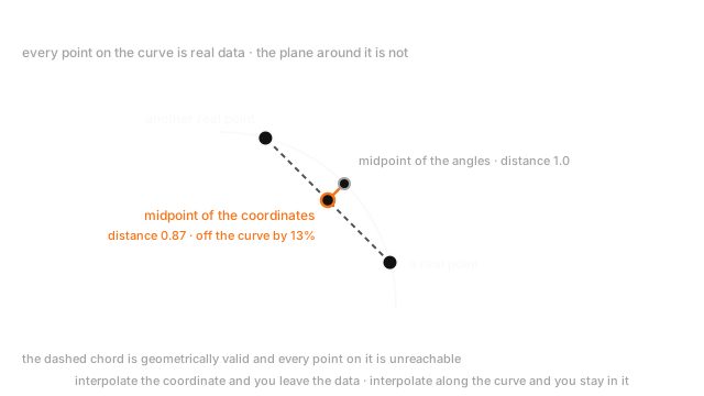
Two real points at 15° and 75°. Average their coordinates and the midpoint sits at distance 0.866 from the centre, not 1.0. It's 13% inside the circle, which is to say it isn't on the manifold and isn't data.

Average their angles instead — 45° — and you get a point at distance exactly 1.0. Still on the circle.

Same two points, same "interpolate halfway" instruction. One route stays in the data and one leaves it, and the only difference is which coordinate system you did the arithmetic in.

Show Me the Code

1import numpy as np2
3theta: np.ndarray = np.array([0.0, np.pi / 2])       # two real points on the unit circle4points: np.ndarray = np.stack([np.cos(theta), np.sin(theta)], axis=1)5
6def radius(p: np.ndarray) -> float:7    """Distance from the centre. On the manifold this is exactly 1."""8    return float(np.linalg.norm(p))9
10chord_mid: np.ndarray = points.mean(axis=0)                              # straight through the plane11arc_mid: np.ndarray = np.array([np.cos(np.pi / 4), np.sin(np.pi / 4)])   # along the manifold12
13print(np.round(points, 3).tolist())        # -> [[1.0, 0.0], [0.0, 1.0]]14print(np.round(chord_mid, 4).tolist())     # -> [0.5, 0.5]15print(round(radius(chord_mid), 4))         # -> 0.7071  off the circle by 29%16print(round(radius(arc_mid), 4))           # -> 1.0     still on it17print(int(round(10_000 * np.log10(256))))  # -> 24082   digits: 10^24082 possible images

chord_mid is a real pair of numbers that is not a member of the set. That's the whole failure mode, in two dimensions where you can see it.

Watch Out For

Interpolating in the input space and calling the result an example

Averaging two rows feels like the obvious way to invent a third. On any curved data distribution it produces points that don't belong to it.

The concrete case is oversampling a minority class by interpolating between neighbours. Two fraudulent transactions differ in amount and hour, and the point between them is a transaction with an amount and an hour that no fraudster ever produced — sometimes sitting squarely inside the legitimate cluster. You've handed the model a mislabelled row and told it to fit it.

Same failure in images. Pixel-averaging two photos gives a double exposure, so training on it teaches the model that ghosts are faces.

Two ways out. Interpolate in a learned latent space, where the coordinates are on the surface. Or interpolate the label along with the input, which is what mixup does and why it works: the model learns "this is 60% cat" rather than "this ghost is a cat".

Reading latent dimensions as attributes, or comparing them across runs

Dimension 7 of your embedding correlates with sentiment across a few hundred examples, so it goes into a dashboard as the sentiment axis.

The space is only defined up to rotation and relabelling. Nothing in the objective asked for one attribute per axis, and unless you trained for disentanglement you almost certainly didn't get it — dimension 7 carries a mixture, and the correlation you found holds on your sample and drifts off it.

The version that breaks pipelines is comparing coordinates across training runs. Retrain with a different seed and dimension 7 means something else entirely, so a stored vector from the old run and a fresh vector from the new one are not comparable, and cosine between them is noise. That's the same versioning rule as vector embeddings: the space belongs to the exact model that produced it.

Probe with a small trained classifier on the whole vector rather than reading axes, and re-embed everything when the encoder changes.

The Quick Version

Real data occupies a tiny, smooth, curved subset of the space that stores it. Sample a 100 × 100 image uniformly and you get static, every time, out of $10^{24082}$ possibilities.
That subset is a manifold, and the intrinsic dimension is how many numbers actually vary — perhaps 30 of the 10,000 you're storing.
A latent space is the coordinate system a model learns on that surface. The encoder maps onto it, the decoder maps back.
A one-pixel shift is enormous in pixel space and tiny in latent space, which is the whole argument for working there.
Interpolating latent codes gives plausible new examples. Interpolating inputs gives a double exposure, because the chord leaves the surface.
On the unit circle, the coordinate midpoint of two points sits 13% inside it. The angle midpoint sits exactly on it.
Off-manifold inputs get confident meaningless answers, which is what adversarial examples exploit and what SMOTE risks.
Reconstruction error is a usable out-of-distribution detector.
Latent axes aren't named attributes, and coordinates from two training runs aren't comparable.