Gen AI

Beam Search

Instead of blindly committing to the best token at each step, keep several parallel universes alive, explore their futures, and prune the paths that score the worst overall.

Beam search keeps multiple candidate sequences alive in parallel, pruning the worst-scoring overall paths at each step

Why Does This Exist?

When an LLM generates text using greedy decoding, it suffers from extreme short-sightedness. At step 1, it picks the token with the highest immediate probability. But this might be a trap. That single word might force the model into an awkward grammatical corner, causing the probabilities at steps 2, 3, and 4 to plummet. If the model had chosen the second-best token at step 1, it might have unlocked a beautifully phrased, high-probability sequence of words later on.

Greedy decoding cannot undo a bad choice. Once a token is selected, it is permanent.

Beam search solves this by refusing to commit. Instead of maintaining one single sequence, it maintains a user-defined number of parallel sequences (the "beam width"). It explores multiple futures simultaneously, sacrificing compute and memory to find the sequence that is mathematically best overall, rather than just best right now.

Think of It Like This

Navigating a maze with clones

Greedy decoding is navigating a maze by walking up to every intersection, looking down the paths, and immediately committing to the one that looks the widest in the first 10 feet. If it turns into a dead end later, you are stuck.

Beam search (with a width of 3) is navigating the maze with clones. At the first intersection, you send 3 clones down the 3 best-looking paths. At the next intersection, all 3 clones split again. You now have 9 clones exploring deep into the maze. You calculate which 3 clones are making the best overall progress, instantly execute the other 6, and repeat. You are exploring the maze in parallel, ensuring you never get permanently trapped by a short-sighted turn.

How It Actually Works

The Expansion and Pruning Cycle

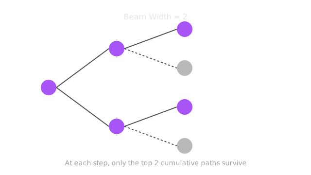
Assume a beam width of $B=2$ .

Initial Step: The model runs a forward pass and looks at the top 2 highest-probability tokens (e.g., "The" at 60%, "A" at 30%). It creates two parallel candidate sequences.
Expansion: For each of the 2 sequences, the model generates the next top 2 tokens. We now have 4 candidate sequences (e.g., "The cat", "The dog", "A cat", "A bird").
Scoring: The system calculates the cumulative probability of all 4 sequences by multiplying the probabilities of their individual tokens (or, in practice, summing their log-probabilities to avoid floating-point underflow).
Pruning: The system sorts the 4 sequences by their cumulative score. It keeps the top 2 and destroys the bottom 2.
The cycle repeats until the surviving sequences hit an <EOS> (End of Sequence) token.

The Memory Cost

Beam search is incredibly expensive. If $B=4$ , the server is functionally running 4 simultaneous generation requests. It must compute the attention matrices and store the KV cache for all 4 sequences in parallel. Modern engines heavily rely on paged attention to make this viable, as the parallel beams can share the exact same physical memory blocks for the parts of their prefixes that haven't diverged yet.

The "Generic" Failure Mode

Beam search is dominant in tasks where there is a single, objectively correct answer (like translating French to English, or summarizing a short factual document).

However, in open-ended creative tasks (like writing a story), beam search is notoriously terrible. Because it ruthlessly optimizes for the highest overall probability, it heavily penalizes rare, interesting words. The resulting text is incredibly safe, bland, and generic. Furthermore, beam search is highly susceptible to infinite loops, often requiring aggressive repetition penalties to force the beams into new vocabulary.

Show Me the Code

This outlines the expansion and pruning logic of a single beam search step using log-probabilities.

1import numpy as np2
3# A sequence is defined by its tokens and its cumulative log-probability4beams = [5    {"tokens": ["The"], "score": np.log(0.60)},6    {"tokens": ["A"],   "score": np.log(0.30)},7]8
9# The model predicts the next step for both beams10# "The" -> "cat" (0.5), "dog" (0.4)11# "A"   -> "cat" (0.9), "bird" (0.05)12predictions = [13    [("cat", 0.5), ("dog", 0.4)],  # Continuations for "The"14    [("cat", 0.9), ("bird", 0.05)] # Continuations for "A"15]16
17expanded_beams = []18
19# 1. Expansion: Create all possible next sequences20for i, beam in enumerate(beams):21    for next_token, prob in predictions[i]:22        new_score = beam["score"] + np.log(prob) # Add log-probs23        new_tokens = beam["tokens"] + [next_token]24        expanded_beams.append({"tokens": new_tokens, "score": new_score})25
26# 2. Pruning: Sort by score descending and keep top B=227expanded_beams.sort(key=lambda b: b["score"], reverse=True)28beams = expanded_beams[:2]29
30for b in beams:31    print(f"Path: {' '.join(b['tokens']):<8} | Score (log-p): {b['score']:.2f}")32
33# -> Path: The cat  | Score (log-p): -1.2034# -> Path: A cat    | Score (log-p): -1.3135# Notice "A cat" (0.3 * 0.9 = 0.27) beat "The dog" (0.6 * 0.4 = 0.24)!36# The model recovered from the fact that "A" was a worse starting word.

By summing the log-probabilities, the algorithm successfully recognized that while "A" was a weaker start, it led to a much stronger continuation, allowing the "A cat" universe to survive the pruning phase.

Watch Out For

Length Bias

Because probabilities are always less than 1.0, multiplying them together (or adding negative log-probabilities) means that longer sequences always have lower scores than shorter sequences. If you run beam search naively, the algorithm will aggressively favor generating very short sentences and stopping immediately. Production implementations always divide the cumulative score by the sequence length (length penalty) to normalize the playing field.

The Quick Version

Greedy decoding makes permanent, short-sighted choices that can ruin a sequence's future probabilities.
Beam search keeps a fixed number of parallel candidate sequences (the beam width) alive simultaneously.
At each step, it expands all candidates, scores their cumulative probability, and prunes the worst performers.
It guarantees a higher-quality overall sequence, making it the industry standard for machine translation and factual summarization.
It is computationally expensive and produces noticeably bland, generic text in open-ended creative writing.