Gen AI

Denoising Diffusion Probabilistic Models

DDPMs generate images by taking pure television static and iteratively removing the noise step-by-step until a clear image emerges.

DDPMs learn to generate data by reversing a Markov chain that slowly corrupts an image into pure Gaussian noise.

Why Does This Exist?

For a long time, the generative AI field was dominated by Generative Adversarial Networks (GANs). GANs could generate incredibly realistic images, but they suffered from mode collapse—meaning they would just memorize a few good examples and produce the same things repeatedly. Furthermore, GANs were notoriously unstable during training.

Denoising Diffusion Probabilistic Models (DDPMs) emerged as a rigorously mathematical alternative that traded the adversarial game for a more stable, thermodynamic-inspired process. Instead of training two neural networks to fight each other, DDPMs rely on a single neural network that learns to perform a very specific task: removing a tiny amount of noise from an image. By chaining this simple denoising operation hundreds of times, a DDPM can start with pure random static and slowly carve it into a highly detailed, coherent image. This process ensures stable training, mathematically predictable likelihoods, and excellent diversity in generated samples, which is why DDPMs quickly became the backbone of modern text-to-image systems.

Think of It Like This

The Sandcastle Sculptor

Imagine building a sandcastle, and then letting the wind slowly blow grains of sand away over several hours until it is nothing but a flat pile of sand. This is the Forward Process: it destroys structure predictably over time.

Now imagine you have a magical assistant who watched this happen, but they only watched in one-second intervals. If you give them a pile of sand, they can estimate where a few grains should go to reverse the last second of wind.

If you ask the assistant to reverse the wind one second at a time, thousands of times in a row, they will eventually rebuild the sandcastle from a flat pile of sand. This is the Reverse Process. The DDPM is the magical assistant learning exactly how to reverse a tiny fraction of the destruction at each step.

How It Actually Works

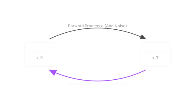
DDPMs are formulated around two opposing Markov chains: the forward process and the reverse process.

1. The Forward Process (Adding Noise)

The forward process, denoted as $q(x_t | x_{t-1})$ , takes a real, clean image $x_0$ and slowly adds Gaussian noise over $T$ steps (where $T$ is typically 1,000). At each step $t$ , a small amount of normally distributed noise is injected according to a variance schedule $\beta_t$ .

Because the sum of Gaussian distributions is also Gaussian, we don't have to simulate this step-by-step to see what the image looks like at step $t=500$ . We can use a mathematical shortcut to jump directly from $x_0$ to $x_t$ using the cumulative variance $\bar{\alpha}_t$ . By the time we reach step $T$ , the image $x_T$ is indistinguishable from pure, isotropic Gaussian noise. The forward process has no learned parameters; it is fixed and deterministic.

2. The Reverse Process (Removing Noise)

The true magic of DDPMs happens in the reverse process, $p_\theta(x_{t-1} | x_t)$ . This process aims to undo the forward process. Because removing noise perfectly is computationally intractable, we use a neural network (typically a U-Net) with parameters $\theta$ to approximate this reversal.

Instead of predicting the clean image directly, the most mathematically robust way to train this network is to predict the noise that was added to the image at step $t$ . The network takes in the noisy image $x_t$ and the current timestep $t$ , and outputs a tensor $\epsilon_\theta(x_t, t)$ representing the noise it believes is present.

3. Training the Network

During training, we sample a random image from our dataset, sample a random timestep $t$ , and generate the noisy version $x_t$ using our forward process shortcut. We then ask the neural network to predict the noise $\epsilon$ . We calculate the Mean Squared Error (MSE) between the actual noise we added and the noise the network predicted. We then backpropagate to update the network weights. This simple objective function naturally weights the loss across different noise levels, leading to stable, highly effective learning.

4. Generation (Inference)

To generate a new image, we start by sampling pure noise from a standard normal distribution to get $x_T$ . We then feed this noise into our trained network, asking it to predict the noise $\epsilon_\theta$ . We subtract a small fraction of this predicted noise to step backward from $t$ to $t-1$ . We repeat this process 1,000 times until we reach $t=0$ . Because the network removes only a tiny fraction of noise at each step, any small prediction errors are corrected in subsequent steps, leading to an incredibly coherent final image.

Show Me the Code

This code demonstrates the simplified training objective of a DDPM, where we sample noise, corrupt the image, and train the model to predict the noise.

1import torch2import torch.nn as nn3
4def ddpm_training_step(model: nn.Module, x_0: torch.Tensor, t: torch.Tensor, alpha_bar: torch.Tensor) -> torch.Tensor:5    """6    Computes the DDPM loss for a single training step.7    8    Args:9        model: The U-Net predicting the noise.10        x_0: Clean batch of images (B, C, H, W).11        t: Randomly sampled timesteps (B,).12        alpha_bar: Cumulative product of (1 - beta) schedule (T,).13    """14    # 1. Sample pure Gaussian noise15    noise = torch.randn_like(x_0)16    17    # 2. Extract the cumulative variance for the current timesteps18    a_bar_t = alpha_bar[t].view(-1, 1, 1, 1)19    20    # 3. Forward process shortcut: compute x_t directly21    # x_t = sqrt(a_bar) * x_0 + sqrt(1 - a_bar) * noise22    x_t = torch.sqrt(a_bar_t) * x_0 + torch.sqrt(1 - a_bar_t) * noise23    24    # 4. Neural network predicts the noise that was added25    predicted_noise = model(x_t, t)26    27    # 5. Compute Mean Squared Error loss between true and predicted noise28    loss = nn.functional.mse_loss(predicted_noise, noise)29    30    return loss31
32# Example usage (mock tensors)33# B=4, C=3, H=64, W=64, T=100034# -> loss (e.g., tensor(0.124))

Watch Out For

Extremely Slow Inference

Because the original DDPM formulation requires passing the image through the neural network 1,000 times sequentially for a single generation, inference is remarkably slow. Unlike a GAN which generates an image in a single forward pass, a DDPM might take seconds or minutes. Modern systems solve this by swapping out the DDPM sampling strategy for faster algorithms (like DDIM) at inference time.

Predicting Noise vs. Image

It might seem intuitive to train the network to predict the clean image $x_0$ directly from the noisy image $x_t$ . While mathematically possible, the original DDPM paper found that predicting the noise $\epsilon$ resulted in vastly superior sample quality because it implicitly scales the learning objective to focus on fine details at lower noise levels.

The Quick Version

DDPMs consist of a forward process (adding noise) and a reverse process (removing noise).
The forward process requires no learning and destroys an image into pure Gaussian noise over $T$ steps.
The reverse process trains a neural network (typically a U-Net) to predict the exact noise added at a specific timestep.
By starting with pure noise and iteratively subtracting the network's predicted noise over hundreds of steps, DDPMs generate diverse, high-quality data.
While training is stable, the step-by-step generative process makes them much slower to sample from than previous architectures like GANs.