Forward & Reverse Processes
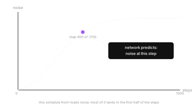
A noise schedule sets how much noise each forward step adds, and at every reverse step the network predicts that added noise, not the clean image itself.
Why Does This Exist?
Diffusion models set up the two-direction shape: a forward process that buries a real image in noise over many steps, and a reverse process that a trained network runs backward to pull an image out of that noise. Fine for a first pass, but it skips two questions that matter once you actually train or sample one of these models.
First: "many steps" of noise — but how much per step? Dump it all in at once and there's no gradual process to learn from. Second: what is the network actually computing at each reverse step? It's tempting to assume it guesses the final image directly, but that's not how the dominant formulation works, and the real answer changes how you read the training code and the sampling loop.
Think of It Like This
Static creeping over a photograph, one frame at a time
Picture a mountain photo on a slowly failing broadcast. At frame 0 it's clean. At frame 1000 it's pure static — no mountain, no sky. Static layers in a little more each frame, following a schedule fixed in advance: maybe it degrades fast early and barely changes near the end, since there's little clean signal left to lose by then.
Now imagine a restorer who's watched this exact degradation thousands of times. Handed a static-choked frame and its frame number, they don't redraw the mountain from scratch — they point and say "here's the static added at this step." Subtract that, and you're one frame closer to clean. Repeat backward from 1000 to 0, and the mountain reappears. That's the reverse process: predict the static, subtract it, step back, repeat.
How It Actually Works
The noise schedule decides where the "hard" work lands
A noise schedule is the plan for how much noise gets mixed in at each of the forward process's fixed number of steps — 1,000 is common. It's a sequence of small values controlling the noise added per step, and their cumulative effect sets how much original signal survives by any given point. Run the mountain photo through a front-loaded schedule, and by step 400 of 1,000 it's already mostly static, with only a faint ridge line and horizon still guessable. That's the mid-schedule point the diagram marks.
The schedule's shape changes what early versus late reverse steps are doing. Front-loaded noise destroys structure fast, so the first reverse steps — working backward from pure noise — are stuck on the coarsest question there is: is this even a mountain-shaped scene at all? The later steps, once rough structure is roughly right, spend their budget on detail — rock texture, sky gradient, where the tree line sits. A schedule that adds noise slowly at first and fast near the end shifts that balance the other way. Neither shape is universally right; it's tuned against the dataset and resolution, and getting it wrong shows up as blurry structure or noisy detail in generated samples.
What the network predicts, concretely
At a given step, the network sees the current noisy mountain photo plus the step number. Its target, in the most common formulation, is not the clean photo — it's the noise component, the specific static mixed in to turn the clean image into this exact noisy one.
That target is convenient because you added it yourself: the forward process's noise at any step is already known during training. Training becomes a plain supervised regression problem — feed in the noisy image and step, ask for the noise, compare against the noise actually added, backpropagate the difference. No indirect signal, no guessing at a final answer hundreds of steps away. Predicting the whole clean image at every step would hand the network a much harder problem, especially early on when almost no structure remains to reconstruct from.
From a noise prediction to a slightly cleaner image
A predicted noise vector alone isn't an image — it has to get used. The reverse step takes the current noisy photo, takes the network's noise prediction for that step, scales it according to the schedule values that generated the forward process, and subtracts it from the current image. The result is the image for the next, slightly less noisy step — not clean yet, just one step further along.
Repeat that operation, once per step, walking from the noisiest step back to zero, and that's the entire reverse process. There's no separate "structure phase" and "detail phase" as distinct algorithms — it's the same predict-and-subtract step run over and over, and the schedule is what makes early repetitions feel like coarse sketching and late ones feel like fine cleanup.
Code
A linear schedule and the cumulative noise fraction it produces at a step — the curve the diagram plots.
import numpy as np
def linear_schedule(steps: int, beta_start: float = 1e-4, beta_end: float = 0.02) -> np.ndarray: return np.linspace(beta_start, beta_end, steps) # noise added AT each step
def noise_fraction_at(betas: np.ndarray, step: int) -> float: signal_kept = np.prod(1.0 - betas[: step + 1]) # cumulative surviving signal return float(1.0 - signal_kept) # the rest is noise
betas = linear_schedule(steps=1000)print(round(noise_fraction_at(betas, step=400), 3)) # -> 0.806, mostly noise by step 400print(round(noise_fraction_at(betas, step=100), 3)) # -> 0.105, still mostly signalThat's the curve in the diagram: a small step leaves the mountain photo mostly intact, and by step 400 it's already mostly gone.
Watch Out For
Assuming the network predicts the clean image at every step
In the standard formulation the target is the noise added at that step, not the final photo. Reading training code with the wrong mental model makes the loss look wrong — it's comparing predicted noise to actual noise, which is correct, not a bug.
Assuming any noise schedule works equally well regardless of resolution
A schedule tuned for small images can front-load noise too aggressively for a large, detailed photo, destroying structure before the model has enough steps to rebuild it. Carrying over a schedule from a different dataset without checking sample quality is a common source of blurry or broken output.
The Quick Version
- A noise schedule sets how much noise gets added at each of the forward process's fixed steps.
- A front-loaded schedule pushes coarse-structure work onto early reverse steps and detail onto later ones.
- The network is most commonly trained to predict the noise added at a step, not the clean image.
- That target is directly computable during training, since the forward process added the noise itself.
- Each reverse step scales and subtracts the predicted noise from the current image to get the next step.