Math

Automatic Differentiation

Frameworks do not solve derivatives symbolically or estimate them numerically — they apply the chain rule mechanically to the operations you actually ran, which is exact and cheap.

Sweeping forwards gives you the derivative of everything with respect to one input, so it costs one pass per parameter; sweeping backwards gives one output with respect to everything, so training needs a single pass

Why Does This Exist?

Nobody has derived the gradient of a modern neural network by hand, and nobody needs to. You write a forward pass in Python and .backward() produces exact gradients for every parameter. That is not magic and it is not symbolic algebra — it is a specific technique with a specific cost model, and knowing the model tells you why some things are fast and others surprisingly are not.

Three concrete payoffs:

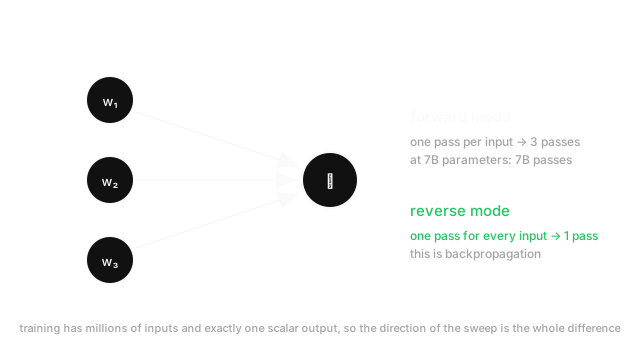
Why training costs about two forward passes, regardless of parameter count. Reverse mode gets every gradient in one sweep. If it scaled per parameter, training a 7-billion-parameter model would be impossible rather than merely expensive.
Why jacrev and jacfwd both exist, and how to pick. Choosing wrong can cost a thousandfold.
Why a custom backward is sometimes necessary, and what you are promising when you write one.

Autodiff is also the reason deep learning research moves quickly: you can change an architecture and get correct gradients without re-deriving anything.

Think of It Like This

Costing a recipe forwards or backwards

A bakery has a chain of steps: flour becomes dough, dough becomes loaves, loaves become a day's revenue.

Ask "if flour gets 1p more expensive, how does everything downstream change?" and you work forwards. Flour price shifts dough cost, which shifts loaf cost, which shifts revenue. One sweep gives you the effect of that one ingredient on every quantity in the chain. To learn about yeast you sweep again.

Ask "revenue dropped — how much did each ingredient contribute?" and you work backwards. Start at revenue, attribute the change to loaves, then to dough, then to every ingredient at once. One sweep, all ingredients.

Both compute the same relationships and their costs are wildly different depending on the shape of your question. Many inputs and one output — which is exactly a loss function over parameters — means backwards wins by the number of inputs.

The catch is that backwards requires you to have kept the intermediate quantities. You cannot attribute revenue to flour without knowing how much dough there was.

How It Actually Works

Autodiff is neither of the two things people assume.

It is not symbolic differentiation. Symbolic tools manipulate expressions and produce formulas, which suffer expression swell — the symbolic derivative of a deep composition is enormous and slow to evaluate.

It is not numerical differentiation. Finite differences approximate, need a step size, cost one evaluation per input, and lose precision to catastrophic cancellation.

Autodiff is exact and cheap because it applies the chain rule to the sequence of operations that ran. Every primitive — add, multiply, exp, matmul — has a known local derivative, and the framework composes them numerically as it goes. No formula is ever produced, and no approximation is made: the result is exact to floating-point precision.

Two directions, one rule

Forward mode propagates derivatives alongside values, from inputs to outputs. Each variable carries a pair: its value, and its derivative with respect to one chosen input. One sweep gives $\partial(\text{everything}) / \partial x_j$ for a single $j$ .

The elegant implementation is dual numbers: represent each quantity as $a + b\epsilon$ where $\epsilon^2 = 0$ . Then ordinary arithmetic propagates derivatives automatically, since $(a + b\epsilon)(c + d\epsilon) = ac + (ad + bc)\epsilon$ — and $ad + bc$ is exactly the product rule.

Reverse mode runs the function forward while recording a computational graph, then walks it backwards accumulating derivatives. One sweep gives $\partial(\text{one output}) / \partial(\text{everything})$ .

The cost model that decides everything

For a function with $n$ inputs and $m$ outputs, in units of one function evaluation:

Forward mode: about $n$ sweeps for the full Jacobian. Cheap when $n$ is small.
Reverse mode: about $m$ sweeps. Cheap when $m$ is small.

Training has $n$ in the billions and $m = 1$ , because the loss is a scalar. Reverse mode gets the entire gradient in one sweep; forward mode would need one per parameter. That asymmetry is the single most important fact about autodiff, and it is why "autodiff" and "backpropagation" are used almost interchangeably in ML even though backpropagation is just reverse mode applied to a network.

The trade is memory. Reverse mode must retain intermediate values for the backward pass, so activation memory scales with depth and batch size. Forward mode needs no tape at all — constant memory — which is why it is used for Jacobian-vector products and for verifying gradients on small inputs.

Where the abstraction leaks

Autodiff is exact for the operations it sees, and three situations break that:

Non-differentiable points. ReLU at exactly zero, abs, max, rounding. Frameworks pick a subgradient by convention and carry on silently. Usually harmless, occasionally not.
Control flow on data. A dynamic framework differentiates the branch that ran, which is correct for that input and means the gradient is only valid locally.
Operations outside the framework. A NumPy call, a C extension, a simulator, or a discrete sampling step has no recorded derivative. The chain silently stops, and you get zero gradient rather than an error.

That last one is the expensive failure, and it is what custom backward implementations and reparameterisation tricks exist to repair.

Worked example

Take $f(x_1, x_2) = x_1 x_2 + \sin(x_1)$ at $(2, 3)$ .

Forward pass, recording each intermediate:

$v_1 = x_1 = 2$
$v_2 = x_2 = 3$
$v_3 = v_1 v_2 = 6$
$v_4 = \sin(v_1) = \sin(2) \approx 0.9093$
$v_5 = v_3 + v_4 \approx 6.9093$

Reverse pass, starting from $\partial f / \partial v_5 = 1$ and walking back:

Addition sends its incoming derivative to both inputs unchanged: $\bar v_3 = 1$ , $\bar v_4 = 1$ .
$v_4 = \sin(v_1)$ has local derivative $\cos(v_1)$ , contributing $\bar v_4 \cos(2) = -0.4161$ to $\bar v_1$ .
$v_3 = v_1 v_2$ has local derivatives $v_2$ and $v_1$ , contributing $\bar v_3 \cdot 3 = 3$ to $\bar v_1$ and $\bar v_3 \cdot 2 = 2$ to $\bar v_2$ .

Note $v_1$ receives contributions from two paths, and they add:

\frac{\partial f}{\partial x_1} = 3 + \cos(2) \approx 3 - 0.4161 = 2.5839, \qquad \frac{\partial f}{\partial x_2} = 2

Verify analytically: $\partial f/\partial x_1 = x_2 + \cos(x_1) = 3 + \cos 2$ ✓ and $\partial f/\partial x_2 = x_1 = 2$ ✓.

The cost comparison is the point. Reverse mode produced both partials in one backward sweep. Forward mode would need two sweeps — one seeded on $x_1$ , one on $x_2$ . With two inputs that is a factor of 2; with 7 billion it is the difference between possible and not.

Show Me the Code

1import math2
3
4class Dual:5    """Forward mode: value plus derivative, propagated by the arithmetic itself."""6
7    def __init__(self, val: float, der: float = 0.0):8        self.val, self.der = val, der9
10    def __mul__(self, o: "Dual") -> "Dual":11        return Dual(self.val * o.val, self.val * o.der + self.der * o.val)12
13    def __add__(self, o: "Dual") -> "Dual":14        return Dual(self.val + o.val, self.der + o.der)15
16
17def sin_dual(d: Dual) -> Dual:18    return Dual(math.sin(d.val), math.cos(d.val) * d.der)19
20
21# Seed the derivative on x1 only: one forward sweep gives df/dx1.22x1, x2 = Dual(2.0, 1.0), Dual(3.0, 0.0)23out = x1 * x2 + sin_dual(x1)24print(round(out.val, 4), round(out.der, 4))      # -> 6.9093 2.583925
26# Seeding x2 instead needs a SECOND sweep — that is the cost of forward mode.27x1, x2 = Dual(2.0, 0.0), Dual(3.0, 1.0)28print(round((x1 * x2 + sin_dual(x1)).der, 4))    # -> 2.029
30print(round(3 + math.cos(2), 4), 2.0)            # -> 2.5839 2.0  analytic check

2.5839 and 2.0 match the hand calculation, and the analytic check confirms them. The two separate seedings are the forward-mode cost made explicit: one sweep per input, where reverse mode would have taken one sweep total.

Watch Out For

Breaking the chain with an operation the framework cannot see

Autodiff only differentiates operations it recorded. Step outside the framework and the chain ends silently.

The routes are ordinary. Converting to NumPy and back with .numpy() or .detach(). Calling a C extension or an external simulator. Using .item() mid-computation. Indexing with a value derived from data in a way that drops the graph. In every case the forward result is correct and the gradient is zero or missing — and a zero gradient is not an error, it is a parameter that never updates.

The symptom is a subset of parameters staying at their initial values while training otherwise proceeds. It is easy to miss because the loss does go down, driven by the parameters that are still connected.

Two defences. Assert that gradients exist and are nonzero after the first backward pass — iterate the parameters and check p.grad is not None and p.grad.abs().sum() > 0. That one loop catches this whole class of bug immediately. And when you genuinely must leave the framework, write a torch.autograd.Function with an explicit backward, then verify it with a numerical gradient check — torch.autograd.gradcheck exists for exactly this and uses float64 because that is what finite differences require.

Discrete sampling is the special case worth naming: sampling from a categorical distribution has no useful gradient, which is why the Gumbel-softmax and REINFORCE exist.

Choosing the wrong mode for the shape of your problem

Forward and reverse mode compute the same derivatives at wildly different costs, and the cost depends only on the input and output counts.

jacrev costs one sweep per output; jacfwd costs one per input. So for a function with 5 inputs and 10,000 outputs, jacfwd is about 2,000 times cheaper — and jacrev is the one people reach for by habit, because reverse mode is what they associate with autodiff.

Reverse mode is right for training because a loss is scalar. It is often wrong for everything else. Sensitivity analysis of many outputs with respect to a few hyperparameters, Jacobians of small dynamical systems, and directional derivatives all favour forward mode. Composing them is also standard practice: jacfwd(jacrev(f)) is the usual way to get a Hessian, because the gradient has many inputs and one output while the second derivative benefits from a forward sweep over it.

Memory is the other axis. Reverse mode holds the whole tape, so peak memory grows with depth. Forward mode holds nothing extra. If you are memory-bound rather than compute-bound on a function with few inputs, forward mode can win outright.

The habit: count $n$ and $m$ before choosing. Fewer outputs means reverse; fewer inputs means forward.

The Quick Version

Autodiff is neither symbolic nor numerical. It applies the chain rule to the operations that actually ran, exactly.
Every primitive has a known local derivative; the framework composes them numerically.
Forward mode: derivatives travel with values, one sweep per input, constant memory. Dual numbers are the clean implementation.
Reverse mode: record a graph forward, walk it back, one sweep per output. Needs the tape, so memory grows with depth.
Cost is $n$ sweeps forward, $m$ sweeps reverse. Training has $n$ in the billions and $m = 1$ .
That is why training costs about two forward passes regardless of parameter count.
Backpropagation is reverse-mode autodiff applied to a neural network.
jacrev scales with outputs, jacfwd with inputs. jacfwd(jacrev(f)) is the standard Hessian.
Gradients arriving by several paths are summed at the node.
The chain breaks silently at NumPy conversions, .detach(), external code and discrete sampling. Assert nonzero gradients after the first step.
Non-differentiable points get a convention, not an error. Verify custom backwards with gradcheck in float64.