Math

Eigenvalues and Eigenvectors

The rare directions a matrix leaves pointing the same way, merely stretched — and the stretch factors that tell you what the matrix really does.

Almost every vector gets rotated when a matrix acts on it; an eigenvector is one of the rare directions that survives untouched and merely gets stretched

Why Does This Exist?

"Just lower the learning rate" is advice you have probably given and received. Eigenvalues explain why it works, why it is unsatisfying, and what the actual problem is.

The curvature of your loss surface in each direction is an eigenvalue of the Hessian. When the largest is 1000× the smallest, any single learning rate is simultaneously too large for the steep directions — where it overshoots and oscillates — and far too small for the shallow ones, where progress crawls. That ratio is the condition number, and it is the real reason training is slow. Adam's per-parameter step sizes are an approximation to fixing it.

The same numbers show up in three more places you use. PCA finds the eigenvectors of the covariance matrix, and their eigenvalues are exactly how much variance each direction carries. The spectral norm of a weight matrix — its largest singular value, which for symmetric matrices is an eigenvalue — is what spectral normalisation constrains in GANs. And PageRank is one long eigenvector computation.

Think of It Like This

Stretching a sheet of rubber

Pin a sheet of rubber to a table and pull it — harder east–west than north–south. Draw arrows on it beforehand and watch what happens.

Most arrows both grow and swing round, because they get pulled more in one direction than the other and end up pointing somewhere new. But two special families do not rotate at all. An arrow lying exactly along the east–west pull just gets longer. One lying exactly north–south also just gets longer, by a different amount. Those are the eigenvectors, and the two stretch factors are the eigenvalues.

Knowing them tells you everything about the stretch, because any arrow can be split into an east–west part and a north–south part, each of which you know how to stretch. A complicated deformation collapses into two independent scalings.

Two extreme cases are worth holding on to. A stretch factor of 1 means that direction is untouched. A factor of 0 means the sheet was crushed flat along that direction, and no amount of pulling recovers what was there.

How It Actually Works

An eigenvector of a square matrix $A$ is a nonzero vector whose direction survives the transformation:

Av = \lambda v

In plain words: applying the matrix to $v$ gives back $v$ scaled by a number. That number $\lambda$ is the eigenvalue. The whole set of eigenvalues is the matrix's spectrum, which is where "spectral" in spectral norm and spectral clustering comes from.

Eigenvectors come in families: if $v$ works, so does any multiple of it, so implementations return unit-length representatives and the sign is arbitrary.

Finding them

Rearrange to $(A - \lambda I)v = 0$ . For a nonzero $v$ to satisfy this, the matrix $A - \lambda I$ must destroy a direction — it must be singular. So:

\det(A - \lambda I) = 0

In plain words: the eigenvalues are exactly the values that make $A - \lambda I$ collapse. Expanding that determinant gives the characteristic polynomial, of degree $n$ , so an $n \times n$ matrix has $n$ eigenvalues counted with multiplicity.

Nobody computes it this way past $2 \times 2$ — root-finding on a degree-1000 polynomial is numerically hopeless. Real implementations use iterative algorithms, and the simplest is worth knowing: power iteration repeatedly multiplies a random vector by $A$ and renormalises. It converges to the dominant eigenvector, because that component grows fastest relative to the others. PageRank is power iteration, and so is the spectral-norm estimate in spectral normalisation, usually with a single iteration per training step.

Two free checks

These catch a large fraction of implementation errors, and both are one line:

\sum_i \lambda_i = \text{trace}(A), \qquad \prod_i \lambda_i = \det(A)

In plain words: the eigenvalues sum to the diagonal total and multiply to the determinant. Always use them when you compute eigenvalues by hand.

Symmetric matrices are the good case

For a symmetric matrix ( $A = A^{T}$ ) three things all become true at once: every eigenvalue is real, eigenvectors of distinct eigenvalues are orthogonal, and the matrix decomposes as

A = Q \Lambda Q^{T}

with $Q$ orthogonal and $\Lambda$ diagonal. This is the spectral theorem, and it is why symmetric matrices are so much nicer to work with.

It matters because the matrices you actually care about are symmetric. Covariance matrices are, which is what makes PCA well behaved and its components orthogonal. Hessians are, which is what makes curvature analysis meaningful. Graph Laplacians and Gram matrices are.

Non-symmetric matrices can have complex eigenvalues — a rotation matrix has no real eigenvector, because no direction survives a rotation. This is the source of a common code surprise, covered below.

What the eigenvalues tell you

Sign — for a symmetric matrix, all positive means positive definite, so a bowl and a minimum. All negative, a maximum. Mixed signs, a saddle. This is exactly how the Hessian classifies a stationary point.
Magnitude — the largest, $|\lambda|_{\max}$ , is the spectral radius, and it governs stability: repeated multiplication grows if it exceeds 1 and decays if it is below. This is the vanishing and exploding gradient story in recurrent networks, stated precisely.
Ratio — the condition number $\kappa = |\lambda|_{\max} / |\lambda|_{\min}$ measures how badly stretched the geometry is. Large $\kappa$ means ill-conditioned: slow optimisation, and sensitivity to small input changes.

Worked example

Take $A = \begin{bmatrix} 2 & 1 \\ 1 & 2 \end{bmatrix}$ , which is symmetric, so expect real eigenvalues and orthogonal eigenvectors.

The characteristic polynomial:

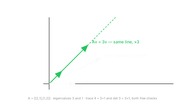
\det \begin{bmatrix} 2 - \lambda & 1 \\ 1 & 2 - \lambda \end{bmatrix} = (2-\lambda)^2 - 1 = \lambda^2 - 4\lambda + 3 = 0

Factoring gives $(\lambda - 3)(\lambda - 1) = 0$ , so $\lambda_1 = 3$ and $\lambda_2 = 1$ .

Check both free identities: trace is $2 + 2 = 4$ and $3 + 1 = 4$ ✓. Determinant is $4 - 1 = 3$ and $3 \times 1 = 3$ ✓.

For $\lambda = 3$ , solve $(A - 3I)v = 0$ , which is $\begin{bmatrix} -1 & 1 \\ 1 & -1 \end{bmatrix} v = 0$ , giving $-v_1 + v_2 = 0$ , so $v = [1, 1]$ . Verify directly: $A[1,1]^{T} = [2+1,\; 1+2]^{T} = [3,3]^{T} = 3[1,1]^{T}$ ✓.

For $\lambda = 1$ : $\begin{bmatrix} 1 & 1 \\ 1 & 1 \end{bmatrix} v = 0$ gives $v_1 + v_2 = 0$ , so $v = [1, -1]$ . Verify: $A[1,-1]^{T} = [2-1,\; 1-2]^{T} = [1,-1]^{T} = 1 \cdot [1,-1]^{T}$ ✓.

The two eigenvectors are orthogonal, as the spectral theorem promised: $[1,1] \cdot [1,-1] = 1 - 1 = 0$ ✓.

Condition number: $3 / 1 = 3$ . Mild. And a non-eigenvector confirms the contrast — $A[2,0]^{T} = [4, 2]^{T}$ , which points in a new direction, exactly as the diagram shows.

Show Me the Code

1import numpy as np2
3A = np.array([[2.0, 1.0], [1.0, 2.0]])            # symmetric4
5vals, vecs = np.linalg.eigh(A)                     # eigh: symmetric, real, ascending6print(vals)                                        # -> [1. 3.]7print(round(vals.sum(), 10), round(np.trace(A), 10))        # -> 4.0 4.08print(round(float(np.prod(vals)), 10), round(np.linalg.det(A), 10))  # -> 3.0 3.09
10v = vecs[:, 1]                                     # eigenvector for lambda = 311print(np.allclose(A @ v, 3 * v))                    # -> True12print(round(float(vecs[:, 0] @ vecs[:, 1]), 10))    # -> 0.0  orthogonal13
14# A rotation has NO real eigenvector, so eig() returns complex values.15R = np.array([[0.0, -1.0], [1.0, 0.0]])16print(np.linalg.eigvals(R))                         # -> [0.+1.j 0.-1.j]17print(round(vals[1] / vals[0], 4))                  # -> 3.0  condition number

Eigenvalues 1 and 3, trace 4, determinant 3, orthogonal eigenvectors — every number matches the hand calculation. The rotation matrix is the complex case from the next section.

Watch Out For

Using eig where eigh belongs

np.linalg.eig handles general matrices and therefore returns complex arrays, in arbitrary order. np.linalg.eigh is for symmetric or Hermitian matrices and returns real values, sorted ascending, using a faster and more accurate algorithm.

Call eig on a covariance matrix and you get eigenvalues like 2.9999999+0.j. They are correct, and they are complex dtype — so downstream comparisons behave oddly, np.sort on complex values sorts by real part then imaginary, plotting libraries warn or silently discard the imaginary part, and any if lambda > 0 test raises or misbehaves. People then chase a phantom bug in their PCA.

There is a subtler version. A matrix that should be symmetric often is not exactly, because floating-point arithmetic in X.T @ X leaves asymmetries around $10^{-16}$ . eig will then hand back genuinely complex eigenvalues with tiny imaginary parts. The fix is to symmetrise explicitly — A = (A + A.T) / 2 — and then call eigh.

Rule of thumb: if the matrix is a covariance, a Gram matrix, a Hessian, or a graph Laplacian, use eigh. Reach for eig only when the matrix genuinely is not symmetric, and then expect complex results as normal rather than as an error.

Reading eigenvalues from a matrix that was never scaled

Eigenvalues carry the units of your data, so they are meaningless across features measured on different scales — and the conclusions you draw from them are then wrong rather than merely imprecise.

The classic case is PCA on unscaled data. Include a feature in metres and another in millimetres and the millimetre feature has a variance a million times larger, so it dominates the covariance matrix, and the first principal component points almost entirely along it. You conclude that feature is the important one, when all you measured was your choice of unit.

Condition numbers suffer identically. An ill-conditioned matrix caused purely by feature scaling looks like a hard optimisation problem, and rescaling fixes it entirely — which is a large part of why feature standardisation speeds up training so reliably. It is not a trick; it is removing artificial anisotropy from the loss surface.

So standardise features before any eigen-based analysis, and when you report an eigenvalue spectrum, report the proportions — each eigenvalue over their sum — rather than the raw values. Proportions are unit-free and comparable; raw eigenvalues are neither.

The Quick Version

$Av = \lambda v$ : an eigenvector keeps its direction, the eigenvalue is the stretch factor. The set of them is the spectrum.
They solve $\det(A - \lambda I) = 0$ , but nobody computes it that way past $2 \times 2$ . Iterative methods, and power iteration for the dominant one.
Two free checks: eigenvalues sum to the trace and multiply to the determinant.
Symmetric matrices give real eigenvalues, orthogonal eigenvectors, and $A = Q \Lambda Q^{T}$ . Covariance, Hessians, Laplacians and Gram matrices are all symmetric.
Non-symmetric matrices can have complex eigenvalues — a rotation has no real eigenvector.
Signs classify a stationary point: all positive is a minimum, mixed is a saddle.
The spectral radius governs stability under repeated multiplication — the exploding/vanishing gradient story.
The condition number $|\lambda|_{\max}/|\lambda|_{\min}$ is why one global learning rate struggles, and what adaptive optimisers approximate away.
Use eigh for symmetric matrices, and symmetrise first if floating point made it slightly asymmetric.
Standardise features first, and report eigenvalue proportions rather than raw values.