Math

Multiple Comparisons

Test enough things at the usual threshold and a false positive stops being unlikely and becomes near certain — which is what every hyperparameter sweep is quietly doing.

Run enough tests at the usual five percent threshold and a false positive stops being unlikely and becomes near certain: by twenty tests the chance of at least one is already sixty-four percent

Why Does This Exist?

You sweep 50 hyperparameter configurations, pick the best validation score, and report it as an improvement. You have just run 50 tests and reported the most extreme result, and the arithmetic says you would find a "winner" that way even if every configuration were identical.

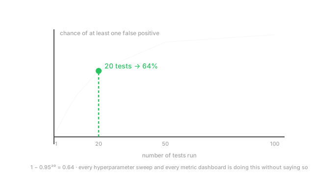
That is not a hypothetical. At $\alpha = 0.05$ and 20 independent tests, the chance of at least one false positive is 64%. At 50 tests it is 92%. The 5% you chose applies to one test, and nothing warns you when you have run more.

Machine learning runs into this constantly and rarely names it:

Hyperparameter sweeps — one test per configuration.
Metric dashboards — checking accuracy, precision, recall, F1 and AUC is five tests.
Per-segment analysis — "it improved for mobile users in Germany" is one test per segment.
Repeated peeking at a running A/B test.

This is the mechanism behind results that look strong in a sweep and land flat in production, and behind the replication crisis in published research.

Think of It Like This

A dart player who only shows you their best throw

Someone claims to be an excellent darts player. They throw one dart and hit the bullseye. That is real evidence.

Now a different scenario: they throw a hundred darts, walk to the board, and photograph only the one nearest the centre. The photograph is identical. The evidence is worthless — with a hundred throws, one landing near the centre is expected from someone with no skill at all.

Nothing about the winning dart changed. What changed is how many attempts you were not told about, and that count is what determines whether the result is surprising.

A hyperparameter sweep is the hundred darts. The winning configuration's score is the photograph. Reporting it without the count of attempts is showing the photograph and omitting the ninety-nine misses — and the fix is not a better dart, it is either declaring the number of throws or holding back a fresh board to throw at once.

How It Actually Works

With $m$ independent tests each at level $\alpha$ , the chance of at least one false positive is:

\text{FWER} = 1 - (1 - \alpha)^{m}

In plain words: the probability none of them falsely fires is $(1-\alpha)^m$ , so one minus that is the probability at least one does. This is the family-wise error rate, and it grows fast:

1 test → 5%
5 tests → 22.6%
10 tests → 40.1%
20 tests → 64.2%
50 tests → 92.3%
100 tests → 99.4%

The expected count of false positives is simply $m\alpha$ , so 20 tests expect one and 100 tests expect five.

Two things you might want to control

Family-wise error rate (FWER) — the probability of any false positive. Strict, appropriate when a single false claim is costly.

False discovery rate (FDR) — the expected proportion of your rejections that are false. More permissive, appropriate when you are screening many candidates and can tolerate some wrong ones because you will follow up.

The choice matters. Confirming a model for production is an FWER situation. Screening 10,000 features for which ones look promising is an FDR situation.

The corrections

Bonferroni — test each hypothesis at $\alpha/m$ . For 20 tests at overall 5%, each must clear 0.0025. Dead simple, controls FWER, valid even when tests are dependent. Its weakness is severity: with many tests it destroys power, so you miss real effects.

Holm–Bonferroni — sort the p-values ascending and compare the $k$ -th against $\alpha/(m - k + 1)$ , stopping at the first failure. Strictly more powerful than Bonferroni, same FWER guarantee, no extra assumptions. There is no reason to use plain Bonferroni over Holm.

Benjamini–Hochberg — sort ascending, find the largest $k$ with $p_k \le \frac{k}{m}\alpha$ , and reject everything up to it. Controls FDR rather than FWER, so it is far more powerful for large $m$ . The standard choice when screening.

The version nobody counts

Formal corrections only help if you know $m$ , and the damaging cases are the ones where nobody was counting:

Trying several metrics and reporting whichever moved.
Slicing by segment until one shows an effect.
Peeking at an A/B test repeatedly and stopping at significance.
Re-running with different seeds and reporting the best.
Adjusting preprocessing and re-evaluating each time.

This is the garden of forking paths, and it inflates the error rate exactly as much as explicit multiple testing does. No correction can fix it after the fact, because the count is unknown.

The structural defence beats any correction: a held-out test set touched exactly once. All the searching happens on validation; the test set is evaluated after every decision is final. That converts an unknown $m$ into $m = 1$ .

Worked example

Twenty independent tests at $\alpha = 0.05$ , no real effects anywhere.

The chance a single test does not falsely fire is $1 - 0.05 = 0.95$ . For all twenty to stay quiet:

0.95^{20} \approx 0.3585

So the chance at least one fires is:

1 - 0.3585 = 0.6415

64%. More likely than not, you will find a "significant" result in a sweep of twenty where nothing is happening. And the expected number of false positives is $20 \times 0.05 = 1$ — you should expect one.

Bonferroni's response is to require each test to clear $0.05/20 = 0.0025$ . Check that it works: $1 - (1 - 0.0025)^{20} \approx 0.0488$ , just under 5% ✓.

Now see the cost. A test with a p-value of 0.01 is significant on its own and not significant after Bonferroni, since $0.01 > 0.0025$ . That is the power you traded away, and with 100 tests the threshold becomes 0.0005 and almost nothing survives — which is why Benjamini–Hochberg exists.

Contrast BH on the same data. With 20 tests and a sorted p-value of 0.01 in position $k = 4$ , the BH threshold is $\frac{4}{20} \times 0.05 = 0.01$ , so it is retained. Same p-value, different guarantee, real difference in what you can detect.

Show Me the Code

1import numpy as np2from statsmodels.stats.multitest import multipletests3
4for m in (1, 5, 10, 20, 50, 100):5    print(m, round(1 - (1 - 0.05) ** m, 4))6# -> 1 0.05 | 5 0.2262 | 10 0.4013 | 20 0.6415 | 50 0.9231 | 100 0.99417
8print(round(0.05 / 20, 4), round(1 - (1 - 0.0025) ** 20, 4))   # -> 0.0025 0.04889
10p = np.array([0.001, 0.004, 0.008, 0.010, 0.030, 0.20, 0.45, 0.60])11for method in ("bonferroni", "holm", "fdr_bh"):12    print(method, multipletests(p, alpha=0.05, method=method)[0])13# bonferroni  [ True  True False False False False False False]14# holm        [ True  True  True False False False False False]15# fdr_bh      [ True  True  True  True  True False False False]16
17# Simulation with NO real effect: how often does a sweep of 20 "find" something?18rng = np.random.default_rng(0)19print(float(np.mean((rng.uniform(size=(20_000, 20)) < 0.05).any(axis=1))))  # -> ~0.642

The simulated 0.642 matches the predicted 0.6415 exactly. The three-method comparison is the power trade made concrete on identical data: Bonferroni keeps 2, Holm keeps 3, and BH keeps 5.

Watch Out For

Correcting for the tests you ran, not the tests you could have

Applying Bonferroni to the 20 configurations in your sweep looks rigorous and usually understates the problem, because the sweep was not the only search.

The real count includes everything you tried on the way: the earlier sweeps that went nowhere, the three preprocessing variants, the two feature sets, the seeds you re-ran, the metrics you checked. If you have been iterating on a problem for a month, the effective $m$ is in the hundreds and there is no honest way to reconstruct it.

Correction methods need $m$ up front, so they cannot rescue a search whose size is unknown. This is why "we corrected for multiple comparisons" is weaker evidence than it sounds.

The defence is procedural, not statistical. Hold out a test set and touch it once, after every choice is final — that makes $m = 1$ by construction and is the only reliable answer. Pre-register the primary metric and the analysis before running the experiment, so the choice cannot be made after seeing results. And report the search size you can account for; a reader who knows you tried 50 configurations can discount appropriately, and one who does not cannot.

Using Bonferroni when the tests are correlated

Bonferroni assumes nothing about dependence, which makes it always valid — and badly conservative when your tests are correlated, which in ML they usually are.

Accuracy, precision, recall and F1 computed on one test set are strongly correlated: they are functions of the same confusion matrix. Treating them as four independent tests and dividing $\alpha$ by four over-corrects, because the effective number of independent tests is closer to one or two. You lose power for nothing.

The same applies to nearby hyperparameter values, which produce nearly identical models, and to overlapping data segments.

Three better options. Holm is uniformly more powerful than Bonferroni with the same guarantee and no extra assumptions — use it as the default instead. Benjamini–Hochberg is valid under positive dependence, which covers most correlated-metric cases, and is far more powerful at large $m$ . And a permutation-based correction estimates the joint null distribution directly, so it accounts for the actual correlation structure rather than assuming the worst case.

The simplest fix is often not statistical at all: pick one primary metric before you start. Then $m = 1$ for the decision, and the others are descriptive context rather than tests.

The Quick Version

$\text{FWER} = 1 - (1-\alpha)^m$ . At $\alpha = 0.05$ : 20 tests give 64%, 50 give 92%, 100 give 99.4%.
Expected false positives is just $m\alpha$ — 20 tests expect one.
FWER controls the chance of any false positive; FDR controls the proportion of rejections that are false.
Bonferroni tests at $\alpha/m$ . Simple, dependence-proof, and severe.
Holm–Bonferroni is uniformly more powerful with the same guarantee. Prefer it to plain Bonferroni, always.
Benjamini–Hochberg controls FDR and is the right tool for screening many candidates.
Hyperparameter sweeps, metric dashboards, per-segment analysis and repeated peeking are all multiple testing.
The garden of forking paths inflates the error rate with an unknown $m$ , and no correction can repair it afterwards.
A held-out test set touched once makes $m = 1$ by construction. That is the real fix.
Bonferroni over-corrects on correlated tests — and accuracy, precision, recall and F1 are highly correlated.
Choosing one primary metric in advance is often better than any correction.