HNSW

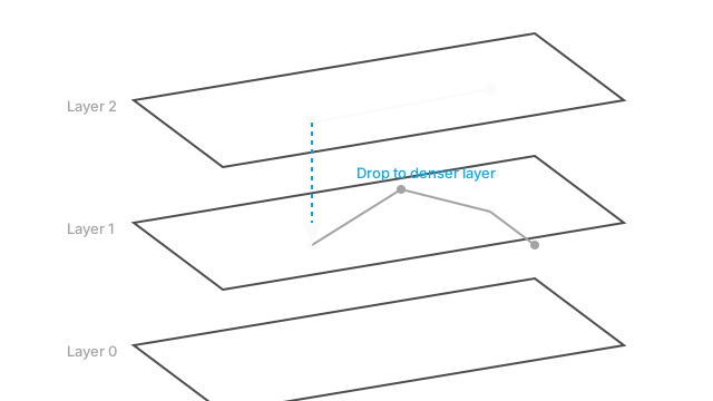
The Problem

Finding the closest vector in a massive dataset (nearest neighbor search) is slow if you check every point. While methods like FAISS (IVF-PQ) partitioned space into clusters, they suffered from edge effects (missing neighbors in adjacent clusters) and search times that grew linearly with the number of clusters checked. Graph-based approaches like Navigable Small World (NSW) were fast but struggled as graphs got extremely large, getting stuck in local "hubs" of densely connected points.

The Idea

The authors introduced Hierarchical Navigable Small World (HNSW). They took the concept of a small-world graph (where you can reach any node in a few hops) and made it hierarchical, heavily inspired by how Skip Lists work for 1D data. By separating links by their length scale into different layers, the algorithm can quickly "zoom in" on the general neighborhood of the query, and then drop to lower layers to find the exact nearest neighbors.

How It Works

HNSW builds a multi-layered graph structure:

1. The Hierarchy: The bottom layer (Layer 0) contains every vector in the dataset, connected to its closest neighbors. As you move to higher layers, points are randomly dropped (exponentially fewer points per layer), leaving only a sparse set of "highway" links.
2. The Search: A search begins at the top, sparsest layer. The algorithm greedily moves to the neighbor closest to the query. Once it hits a local minimum at that layer, it drops down to the exact same point in the layer below.
3. Zooming In: In the lower, denser layer, the search resumes. Because it started near the target (thanks to the layer above), it takes very few hops to find the new local minimum. This repeats until it hits Layer 0, where it performs the final, fine-grained search.

This separation of scales ensures logarithmic search time complexity O(log N).

Why It Mattered

HNSW proved to be astonishingly fast and highly accurate, generally dominating speed/recall benchmarks for Approximate Nearest Neighbor (ANN) search. It became the default indexing algorithm for almost every modern vector database (Pinecone, Qdrant, Milvus, Elasticsearch, pgvector).

What Came After

While HNSW is the undisputed king of in-memory search, its main drawback is massive memory consumption (storing all the graph edges takes more RAM than the vectors themselves). Subsequent research focused on compressing HNSW graphs or combining HNSW with disk-based retrieval (like DiskANN) to handle datasets too large for RAM.