Vector Database (Semantic Search Engine)
AdvancedOn this page
Overview
A Vector Database (like Pinecone, Milvus, or Qdrant) is specialized for storing and querying high-dimensional vectors (embeddings) generated by AI models. Unlike traditional SQL databases that rely on exact row matching, a vector database performs similarity searches—finding data that means the same thing conceptually. It powers RAG applications, image search, and recommendation engines.
Functional Requirements
- Insert, update, and delete dense vectors along with metadata (e.g., doc_id, text_chunk).
- Perform Approximate Nearest Neighbor (ANN) search given a query vector.
- Support hybrid search: filtering by metadata (e.g., 'category=books') before or after the vector search.
- Ensure high recall (the percentage of true nearest neighbors found).
Non-Functional Requirements
- Low latency: search millions of vectors in < 50ms.
- High throughput: support thousands of concurrent search queries.
- Scalability: handle billions of vectors (terabytes of RAM/SSD) by sharding data across nodes.
- Durability: vector indexes must persist across node failures.
Capacity Estimation
Assume a dataset of 1 Billion vectors, each with 1,536 dimensions (e.g., OpenAI embeddings).
- Storage: 1,536 dimensions * 4 bytes (float32) = ~6 KB per vector. 1 Billion vectors = 6 Terabytes of raw vector data.
- Index RAM: Graph-based indexes (like HNSW) require keeping data in memory for speed. 6TB cannot fit on one machine. The data must be sharded across a cluster of ~20-30 memory-optimized nodes (e.g., 256GB RAM each).
- Query Compute: Calculating cosine similarity for billions of vectors via brute force is impossible. The system must use hierarchical indexing to only compute distances for a small fraction of the database.
High-Level Architecture
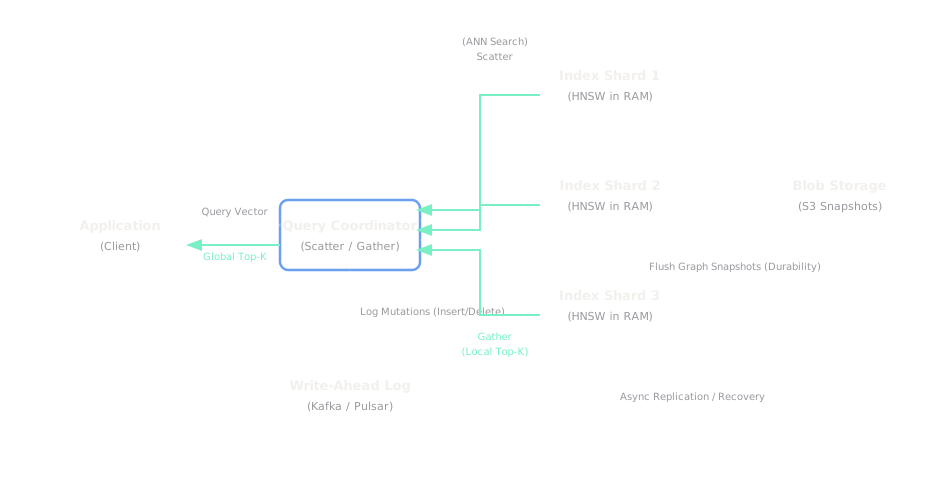
The system is split into two planes: the Control Plane (Metadata) and the Data Plane (Search Nodes). When a query vector arrives at the API Gateway, it routes to a Query Router (Coordinator). The Coordinator scatters the query to all active Shard Nodes. Each Shard Node maintains an HNSW (Hierarchical Navigable Small World) index in memory. The node traverses the HNSW graph to find its local top-K nearest neighbors and returns them to the Coordinator. The Coordinator merges the results, sorts them, and returns the global top-K to the client. Background workers continuously flush new inserts to Write-Ahead Logs (WAL) and blob storage (S3) for durability.
Data Model
| Entity | Fields / Schema | Storage Choice |
|---|---|---|
| vector_index | vector_id, float_array[1536], metadata (JSON) | In-Memory HNSW Graph / SSD (Memory-mapped) |
| write_ahead_log | transaction_id, operation (insert/delete), payload | Distributed Log (Kafka / Pulsar) |
| snapshots | shard_id, index_file_blob | Object Storage (S3 / GCS) |
Detailed Design
The HNSW Index
HNSW is the industry standard algorithm for Approximate Nearest Neighbor (ANN) search. It works like a skip-list for graphs. It creates multiple layers of graphs. The top layer has very few nodes (long jumps). The query starts at the top, finds the closest node, drops down a layer, and repeats until it hits the bottom layer (the dense graph). This reduces query time from O(N) to O(log N).
Metadata Filtering (Pre-filtering vs. Post-filtering)
Users often want to query: "Find vectors similar to X, but ONLY where status='active'".
- Post-filtering: Find the top 100 nearest neighbors first, then discard those where status != 'active'. Problem: If 99 of the 100 are inactive, the user only gets 1 result. (Low recall).
- Pre-filtering: Filter the exact metadata IDs first, then restrict the HNSW traversal to only those IDs. Problem: If the filter is too restrictive, the graph traversal breaks because nodes are missing. Modern databases use dynamic switching between pre/post filtering or single-stage filtering algorithms.
Vector Quantization (Cost Reduction)
Keeping 6TB of float32 vectors in RAM is expensive. Systems use Product Quantization (PQ) or Scalar Quantization to compress vectors from 32-bit floats to 8-bit integers or binary code. This shrinks RAM usage by 4x-10x with only a ~2-5% drop in accuracy.
Bottlenecks & Solutions
The primary bottleneck is Memory Bandwidth and RAM Cost. Graph traversal inherently causes random memory access patterns, which defeats CPU cache lines. Sharding helps distribute the RAM load. Additionally, databases are moving toward DiskANN-style architectures that keep the graph topology in RAM but store the heavy vector payloads on fast NVMe SSDs, drastically lowering hosting costs.