Convolution Operation
One small grid of weights slides across the whole input, multiplying and summing at every position — the same small set of weights, reused everywhere.
Why Does This Exist?
Feed a 200×200 grayscale photo into a plain fully-connected layer and every one of its 40,000 pixels gets its own weight, for every unit in the next layer. Ten thousand units in that layer and you're already past 400 million weights, before the network has done anything except look at one small image once.
That number is the wall, but it's not even the worst part. A weight sitting under the pixel at position (10, 10) has no relationship to the weight sitting under (10, 11). If the network learns to detect a vertical edge at one location, it has to separately relearn that exact same pattern at every other location a vertical edge might appear — which, in a photo, is everywhere. Nothing about "this is an edge" gets shared across the image.
Convolution is the fix, and it's a strange one the first time you see it: instead of one weight per pixel, use a tiny grid of weights — commonly 3×3 or 5×5 — and slide that same tiny grid across the entire input. One shape, reused at every position. That single decision is why a network can look at a photo at all.
Think of It Like This
A rubber stamp, pressed again and again
A rubber stamp carries one fixed pattern. Press it in the top-left corner of a page, lift it, move it one inch right, press again. The ink pattern that comes out depends on what was under the stamp each time — but the stamp itself never changes shape.
A convolution kernel is that stamp. Its nine numbers (for a 3×3 kernel) are fixed once training finishes. Slide it over every position in the input, and at each one it presses down and produces a single number: how strongly the pattern under it matches the pattern baked into the stamp. Do that everywhere, and you get a whole new grid — one number per position, all produced by the same nine weights.
How It Actually Works
One position, one dot product
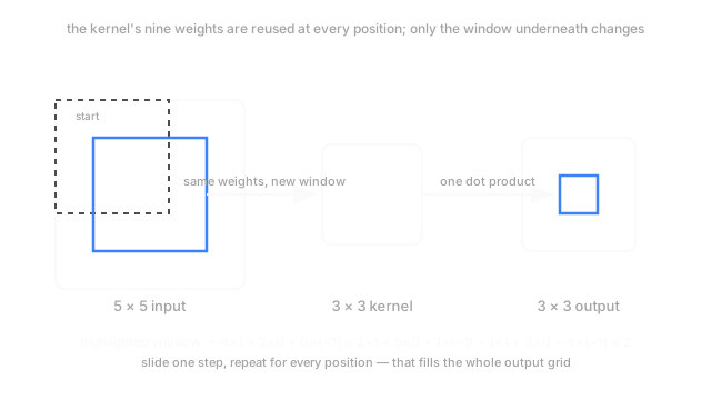
At each position, the kernel overlaps a patch of the input exactly its own size. Multiply every overlapping pair of numbers, then add them all up — that's a dot product, and it's the entire operation. In the diagram above, the highlighted 3×3 patch of the input is [[4,2,0],[2,5,1],[1,3,4]], and the kernel is [[1,0,-1],[1,0,-1],[1,0,-1]]. Multiply position by position and sum: . That single number becomes one cell of the output.
Slide the kernel one column right, recompute, write the next output cell. Finish a row, drop down one row, keep going. A 5×5 input with a 3×3 kernel, moved one step at a time, visits nine positions and produces a 3×3 output — every cell computed by the identical nine weights.
The three knobs that change the shape
Stride is how far the kernel jumps between positions. Stride 1 visits every possible position; stride 2 skips every other one, halving the output's height and width and cutting computation to match.
Padding adds a border of zeros around the input before sliding starts. Without it, a kernel bigger than 1×1 shrinks the output every time it's applied — a 5×5 input with a 3×3 kernel produces a 3×3 output, not 5×5. Pad by 1 pixel on each side first and the output comes back out at 5×5, which is what "same" padding means in most frameworks. The general formula, for input size , kernel size , padding , and stride :
Dilation spreads the kernel's own cells apart, inserting gaps between them so a 3×3 kernel with dilation 2 reads from a 5×5 footprint while still only holding nine weights. It's how a network grows its view of the input without adding a single parameter — the subject of receptive fields.
Weight sharing is the actual idea
Everything above is mechanism. The idea underneath it is that the same nine weights get applied at every position, which is a deliberate assumption: whatever pattern is worth detecting in one part of the image is worth detecting, with the identical detector, in every other part. That assumption is called translation invariance, and it's true for most things a camera photographs — an edge is an edge wherever it falls in the frame.
Compare the weight count directly. A fully-connected layer mapping a 200×200 image to another 200×200 map needs one weight per input-output pixel pair: 1.6 billion. A 3×3 convolutional layer producing the same size map needs nine. Every position benefits from every training example, because every position is trained by the same nine numbers — not just the examples where a pattern happened to land at that exact spot.
Many kernels, not one
A real convolutional layer doesn't apply a single kernel — it applies many, each initialized differently and each learning to respond to a different pattern: one for vertical edges, one for a particular texture, one for a corner. Each kernel produces its own output grid, called a channel, and the layer's true output stacks all of them together. A layer with 64 kernels turns a single-channel input into a 64-channel output, one channel per detector.
Code
The same 5×5 input and kernel from the diagram, computed by hand with nested loops rather than a library, so every multiply-and-sum is visible.
import numpy as np
def conv2d(x: np.ndarray, kernel: np.ndarray) -> np.ndarray: kh, kw = kernel.shape oh, ow = x.shape[0] - kh + 1, x.shape[1] - kw + 1 # stride 1, no padding out = np.zeros((oh, ow)) for i in range(oh): for j in range(ow): patch = x[i : i + kh, j : j + kw] # the window under the kernel right now out[i, j] = float(np.sum(patch * kernel)) # elementwise multiply, then add return out
x = np.array([[3, 1, 0, 2, 1], [1, 4, 2, 0, 1], [0, 2, 5, 1, 0], [2, 1, 3, 4, 2], [1, 0, 2, 1, 3]], dtype=float)vertical_edge = np.array([[1, 0, -1], [1, 0, -1], [1, 0, -1]], dtype=float)
print(conv2d(x, vertical_edge))# -> [[-3. 4. 5.]# [-7. 2. 7.]# [-7. -3. 5.]]Every entry above matches what the diagram's highlighted window produces at position (1, 1): 2.0. Swap vertical_edge for a different 3×3 grid and the same nine multiply-and-sum steps detect something else entirely — the loop never changes, only the numbers inside the kernel.
Watch Out For
Forgetting the kernel is flipped in true convolution
Signal-processing convolution technically flips the kernel before sliding it — mathematically, , and that flip matters for its algebraic properties, like being commutative. Every deep learning framework skips the flip and calls the result "convolution" anyway; what they actually compute is cross-correlation.
This is almost never a problem in practice, because the kernel's weights are learned from random initialization — a network trained with the "wrong" (unflipped) convention simply learns the mirror image of the pattern it would have learned otherwise, and either way it works. It matters only if you're comparing a from-scratch implementation against a signal-processing textbook and the signs come out backwards.
Padding with anything other than the assumption you intend
Zero-padding is the default, and it quietly asserts that "nothing" is the right value for the world outside the image. For most photos that's a reasonable approximation near the edge. For data where the border carries real information — a spectrogram where silence is not zero, or a satellite tile where the edge continues into a neighboring tile — zero-padding introduces a border artifact the network has to learn to ignore, which it does imperfectly.
Reflection padding (mirroring the edge pixels) or replication padding (repeating the last pixel) are both one line to switch to, and either removes the artificial edge zero-padding invents. Check which your framework defaults to before assuming.
The Quick Version
- A kernel is a small fixed grid of weights. Slide it across the input; at each position, multiply overlapping values and sum them — one dot product per position.
- The same weights are reused at every position. That's weight sharing, and it's what makes convolution parameter-efficient and translation-invariant.
- Stride controls how far the kernel jumps between positions; padding controls the output size and what happens at the border; dilation spreads the kernel's own cells apart.
- A real layer applies many kernels in parallel, each producing its own output channel — one detector per channel.
- Frameworks compute cross-correlation and call it convolution. The kernel isn't flipped, and it essentially never matters.