Core ML

Exponential Smoothing

A time series forecasting method that predicts the future by taking a weighted average of past observations, where recent observations are given exponentially more weight than older ones.

Why Does This Exist?

The simplest way to forecast tomorrow's sales is to calculate the average of your sales over the last 30 days. This is a Simple Moving Average.

However, simple moving averages have a fatal flaw: they treat all data points equally. If your business launched a massive ad campaign yesterday, yesterday's sales are far more indicative of tomorrow's sales than the sales from 29 days ago.

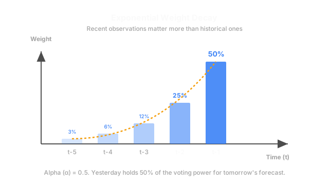
Exponential Smoothing solves this by applying a mathematical decay. It still averages the past, but it assigns the largest weight to the most recent observation, with the weights decaying exponentially the further back in time you look.

Think of It Like This

Imagine you are trying to guess how much your friend will enjoy a new sci-fi movie.

You ask them to rate the last 10 movies they watched.

A Simple Moving Average treats their opinion of a movie they watched 5 years ago as exactly equal to their opinion of a movie they watched yesterday.
Exponential Smoothing assumes their taste changes over time. It weights their review of yesterday's movie at 50%, last week's movie at 25%, last month's movie at 12.5%, and so on. It relies heavily on their current mood while keeping a faint memory of their historical taste.

How It Actually Works

Exponential smoothing is often called ETS (Error, Trend, Seasonality). There are three distinct levels of exponential smoothing, depending on the complexity of your data.

1. Simple Exponential Smoothing (SES)

Use this if your data has no trend and no seasonality (a flat line with noise). It relies on a single smoothing parameter, $\alpha$ (alpha), which sits between 0 and 1.

If $\alpha = 0.9$ , the model reacts violently to recent changes (remembering almost nothing of the past).
If $\alpha = 0.1$ , the model is highly smoothed and stubborn, relying mostly on historical averages. $\text{Forecast} = \alpha \cdot Y_{t} + (1-\alpha) \cdot \text{Previous Forecast}$

2. Double Exponential Smoothing (Holt's Linear Trend)

If your data has a trend (heading up or down over time), SES will constantly lag behind the data, always under-predicting an upward trend. Double exponential smoothing fixes this by adding a second equation to explicitly smooth and forecast the slope of the trend, using a second parameter, $\beta$ (beta).

3. Triple Exponential Smoothing (Holt-Winters)

If your data has both a trend and seasonality (e.g., spikes every December), you must use Holt-Winters. It adds a third equation to smooth the seasonal component, controlled by a third parameter, $\gamma$ (gamma).

Because Holt-Winters explicitly models the Level, Trend, and Seasonality separately, it is mathematically identical in spirit to Time Series Decomposition.

Show Me the Code

In Python, statsmodels provides an ExponentialSmoothing class that can handle SES, Holt's, and Holt-Winters.

1import pandas as pd2import numpy as np3from statsmodels.tsa.holtwinters import ExponentialSmoothing4
5# Dummy monthly data with an upward trend and yearly (m=12) seasonality6data = [10, 12, 15, 20, 25, 30, 28, 22, 18, 15, 12, 11,7        15, 18, 20, 25, 30, 35, 33, 27, 23, 20, 17, 16]8
9# Fit a Triple Exponential Smoothing (Holt-Winters) model10# We specify that both the trend and seasonality are 'additive'11model = ExponentialSmoothing(12    data, 13    trend='add', 14    seasonal='add', 15    seasonal_periods=1216)17fitted_model = model.fit()18
19# Forecast the next 12 months20forecast = fitted_model.forecast(12)21print("Forecast for Year 3:\n", np.round(forecast, 1))22
23# Let the library tell us what optimal Alpha, Beta, and Gamma it found24print(f"Alpha (Level): {fitted_model.params['smoothing_level']:.3f}")25print(f"Beta (Trend): {fitted_model.params['smoothing_trend']:.3f}")26print(f"Gamma (Seasonal): {fitted_model.params['smoothing_seasonal']:.3f}")

Watch Out For

Damped Trends. If your data has been trending upwards at 20% year-over-year, Double Exponential Smoothing will enthusiastically forecast that it will grow at 20% forever until it reaches infinity. In the real world, trends flatten out. You should almost always enable the damped_trend=True parameter in your code, which adds a $\phi$ (phi) parameter to slowly flatten the forecasted trend over time.

The Quick Version

Exponential smoothing predicts the future by averaging the past, but gives exponentially more weight to recent data.
Simple Exponential Smoothing: For data with no trend or seasonality.
Double (Holt's): For data with a trend.
Triple (Holt-Winters): For data with both a trend and seasonality.
It is computationally much cheaper and faster to run than ARIMA, making it the default choice when you need to forecast thousands of distinct metrics simultaneously.

Related concepts

ARIMA