Core ML

Gradient Boosting

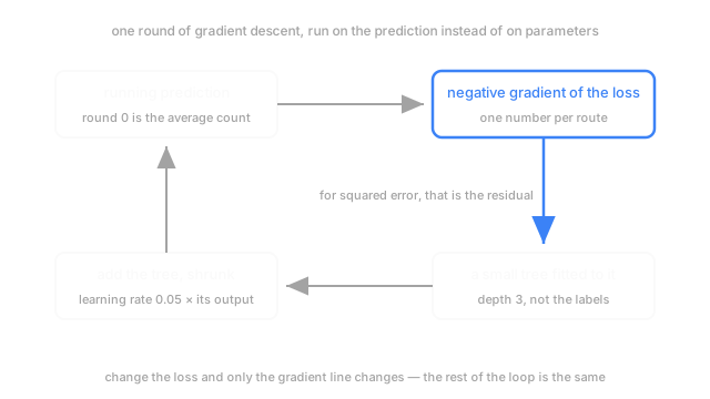
Ordinary gradient descent nudges parameters. Gradient boosting nudges the prediction itself, one small tree per step, fitted to the gradient of your loss.

Each round reads the negative gradient of the loss at the current prediction, fits a small tree to those per-row numbers, and adds a shrunken copy of it back

Why Does This Exist?

Boosting told you to fit each learner to what the previous ones got wrong. It never defined "wrong", and that gap is this page.

Here's the case we'll carry down. A parcel depot wants tomorrow's redelivery count for each of its 400 routes. Most come back with nought, one, two; a route with a broken buzzer on a tower block comes back with forty. You want the number, not a yes-or-no.

Subtract the prediction from the truth, fit the next tree to that difference, and you've silently chosen squared error — which puts a route that missed by 30 at nine hundred times the priority of one that missed by one. On skewed counts that's the wrong instruction. AdaBoost is no help either: its reweighting speaks one loss, exponential, and only for labels of $-1$ and $+1$ .

Friedman's fix, published in 2001, is a change of definition. "What it got wrong" becomes the gradient of whatever loss you chose, evaluated at the current prediction, one number per row.

Think of It Like This

Fixing a boomy hall: knobs versus a measured curve

A hall's PA sounds muddy, and there are two ways at it. Turn the amplifier's eight knobs, broad and overlapping, and guess which owns the boom. That's working on the controls.

Or measure. Play a sweep, read the response at every frequency, and now you have a number at each one saying this band is 6 dB too loud — the fix described directly, in the units of the output.

You can't install a filter per frequency, so you build the closest thing available, a few bands tracing that shape, and apply it at a fraction of full strength, because the measurement is noisy and overshooting is worse than undershooting. Then sweep again.

Sweep, measure, add a shrunken correction, repeat. The measurement is the gradient.

How It Actually Works

Descending on the output instead of the knobs

Gradient descent moves parameters: work out how the loss changes as each one changes, then step against it. Gradient boosting keeps that logic and points it elsewhere, asking what change to the prediction for this row would lower the loss. For row $i$ at round $m$ :

r_{im} = -\left[\frac{\partial L(y_i, F(x_i))}{\partial F(x_i)}\right]_{F = F_{m-1}}

$L$ is your loss, $y_i$ the truth for row $i$ , $F_{m-1}$ the ensemble built so far, and $r_{im}$ the direction that row's prediction wants to move. One number per route, per round.

Take squared error, $L = \tfrac{1}{2}(y - F)^2$ . Its derivative with respect to $F$ is $-(y - F)$ , so the negative gradient is exactly the residual. That's why "fit the next tree to the residuals" is the version everybody remembers: it's this recipe with one loss substituted in.

You can't add those 400 numbers to the model directly — a per-row correction only fixes rows you've seen. So fit a small tree to them, collapsing 400 loose corrections into a handful of leaf values defined by feature ranges, which is what makes them apply to tomorrow's routes. Then $F_m = F_{m-1} + \eta\,h_m$ , with $\eta$ the learning rate and $h_m$ that tree.

The part that buys you everything

Nothing in the loop cares which loss produced the gradients.

Log loss gives you classification, its gradient being label minus predicted probability. Poisson deviance handles counts on a log scale, so it can't predict a negative redelivery. Quantile loss predicts the 90th percentile rather than the mean, which is what the depot wants when it's sizing a van. Huber loss is squared error near zero and absolute error in the tail, so one forty-parcel route stops dominating.

One line changes. That's the reframe AdaBoost triggered, cashed in.

Three dials, and what each one does

The learning rate $\eta$ scales every tree before it's added, so smaller means more rounds for the same fit and better generalisation. Set it low and leave it. The round count isn't tuned directly: fix $\eta$ , watch validation error, stop when it turns up. Tree size decides how many features can interact — depth 1 is additive, depth 3 lets three combine (postcode density with day of week with parcel size), and past six you're usually buying variance.

One borrowing from bagging. Stochastic gradient boosting fits each round on a random 50–80% of rows, often a random subset of columns too, for the reason a random forest does it: decorrelate the members. It regularises and runs faster, a rare pairing.

Show Me the Code

The same four-line loop run twice, with only the gradient swapped: counts under squared error, then a binary flag under log loss.

1import numpy as np2
3rng = np.random.default_rng(4)4x = rng.uniform(0.0, 1.0, 400)5leaf = np.digitize(x, np.quantile(x, [0.25, 0.5, 0.75]))            # stands in for a 4-leaf tree6parcels = rng.poisson(np.exp(0.2 + 3.0 * x)).astype(float)          # redeliveries per route7missed = (rng.uniform(size=400) < 1 / (1 + np.exp(1.5 - 3.0 * x))).astype(float)8
9def descend(y: np.ndarray, loss: str, eta: float = 0.1, rounds: int = 60) -> np.ndarray:10    f = np.full(400, y.mean() if loss == "squared" else 0.0)        # a constant, then corrections11    for _ in range(rounds):12        g = y - f if loss == "squared" else y - 1 / (1 + np.exp(-f))  # negative gradient, per row13        f = f + eta * np.array([g[leaf == k].mean() for k in leaf])   # one tree fitted to it, shrunk14    return f15
16resid = parcels - descend(parcels, "squared")17p = 1 / (1 + np.exp(-descend(missed, "logistic")))18print(f"counts: rmse {parcels.std():.2f} -> {np.sqrt((resid ** 2).mean()):.2f} | flags: log loss 0.693 -> {-(missed * np.log(p) + (1 - missed) * np.log(1 - p)).mean():.3f}")19# -> counts: rmse 7.25 -> 3.42 | flags: log loss 0.693 -> 0.597

Two different problems, one loop, and the only line that knows the difference is the gradient. The 0.693 is $\ln 2$ : the log loss of guessing a coin flip everywhere.

Watch Out For

Leaving the learning rate high and tuning the round count instead

The default rate in most libraries is 0.1 or 0.3, and the round count looks like the interesting parameter. So people grid-search rounds at 0.3 and ship whatever won.

That lands on a coarse model: at 0.3 each tree moves the prediction a long way, so the ensemble steps past the minimum and back, and two runs on slightly different data end up meaningfully apart. Set the rate to 0.05, turn on early stopping, and let it run as long as it needs. Smoother fit, less variance between reruns, and it costs only compute.

Boosting squared error onto a target that isn't shaped like it

Squared error assumes your errors are symmetric and roughly the same size everywhere. Redelivery counts are neither: bounded below by zero, mostly tiny, occasionally enormous, with variance that grows with the mean.

Boost squared error onto that and the model spends its capacity chasing tower blocks, predicts 2.5 where the truth is almost always 0 or 1, and will happily return a negative count. A Poisson objective — one argument in every serious library — fits on a log scale, so predictions stay positive and errors are judged against the expected count. For long-tailed money with a spike at zero, Tweedie is the same idea. Pick the loss from the target's shape first.

The Quick Version

Gradient boosting is gradient descent in function space: the thing being stepped is the prediction, not a parameter vector.
Each round takes the negative gradient of the loss at the current prediction, fits a small tree to those per-row numbers, and adds it scaled by the learning rate.
The tree is what makes the correction generalise; raw per-row gradients only fix rows you've seen.
For squared error the negative gradient is the residual — hence "fit the residuals". One case, not the definition.
Any differentiable loss works: log loss for classes, Poisson for counts, quantile for intervals, Huber for outliers.
Small learning rate, rounds chosen by early stopping, depth 3 to 6. Depth is how many features get to interact.
Subsampling rows and columns each round regularises and speeds things up, borrowed from bagging.