Core ML

Graph Neural Networks

Each node collects information from its neighbors, combines it with its own, and repeats — so a network can learn from relationships, not just isolated rows.

A center node collects messages from each of its neighbors and combines them into a new representation, and stacking this step over more layers lets information travel further across the graph

Why Does This Exist?

A social platform wants to predict which accounts are bots. Each account has its own features — post frequency, account age, profile completeness — and an ordinary classifier trained on those features alone gets most of it right, then misses an entire coordinated cluster: a hundred accounts that individually look plausible but that all follow each other, share the same three links, and joined within the same hour.

That pattern lives in the connections, not in any single account's row of features. A model that only sees rows independently, one at a time, has no way to see it. What's missing is the graph itself — who follows whom — and a way to let each account's prediction depend on its neighbors, not just on itself.

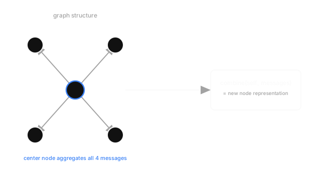
A graph neural network folds the connections into the model directly. A node's representation gets built from its own features plus a summary of its neighbors' representations, and stacking that step means information from two, three, or more hops away eventually reaches every node.

Think of It Like This

Rumors spreading through a group chat, one round at a time

A rumor starts with one person, who tells it to everyone directly connected to them. Next round, each of those people combines what they just heard with what they already knew, and pass their updated version along to their own connections. After a few rounds, someone three friends removed from the original source has an opinion shaped by that far-off event, blended with everything closer to them.

That's message passing: each round, everyone updates using what their direct connections told them last round, and stacking rounds is what lets information travel further than one hop.

How It Actually Works

One layer is one round of message passing

A graph neural network layer does the same two things at every node, simultaneously: gather messages from each neighbor, then combine those messages with the node's own current representation to produce its next one.

h_v^{(k+1)} = \text{combine}\Big(h_v^{(k)},\ \text{aggregate}\big(\{h_u^{(k)} : u \in \mathcal{N}(v)\}\big)\Big)

$h_v^{(k)}$ is node $v$ 's representation after $k$ layers, $\mathcal{N}(v)$ is its set of neighbors, aggregate combines the neighbors' messages into one vector — commonly a sum, mean, or max, since the neighbor count varies node to node and the aggregator has to handle any number — and combine merges that with the node's own state. $h_v^{(0)}$ starts as the node's raw input features.

GCN, GraphSAGE, and GAT differ in how they aggregate

A Graph Convolutional Network (GCN) aggregates by taking a normalized average over neighbors, weighting by how many connections each neighbor itself has, which keeps high-degree nodes from dominating. GraphSAGE samples a fixed-size subset of neighbors per node rather than using all of them, which matters directly for scale — a node with ten thousand connections doesn't need ten thousand messages every layer, and sampling caps that cost regardless of how connected any single node is. A Graph Attention Network (GAT) replaces the fixed averaging with a learned attention weight per neighbor, so the aggregation itself decides which neighbors matter most for a given node instead of treating them equally.

Why depth doesn't help forever: over-smoothing

Stacking convolutional layers in a vision network reliably improves it, up to a point. Stacking graph neural network layers behaves differently: past roughly three to four layers, performance often gets worse, not just stops improving. Each layer mixes a node's representation with its neighbors' — average over a moderate radius and detail sharpens; keep averaging past that radius and every node's representation converges toward the same value, since in a connected graph enough rounds of averaging eventually blends everyone together. This is over-smoothing, and it's the specific reason most practical graph neural networks stay shallow, unlike the very deep stacks that work well for images.

Show Me the Code

Repeatedly averaging each node with its neighbors on a small ring graph, watching the per-node values converge toward the same number.

1import numpy as np2
3n_nodes = 84A = np.zeros((n_nodes, n_nodes))5for i in range(n_nodes):6    A[i, (i - 1) % n_nodes] = 1  # ring: each node connects to 2 neighbors7    A[i, (i + 1) % n_nodes] = 18    A[i, i] = 1  # self-loop, so a node's own value survives averaging9P = np.diag(1.0 / A.sum(axis=1)) @ A  # row-normalized averaging operator10
11rng = np.random.default_rng(0)12x = rng.normal(0, 1, size=(n_nodes, 1))13print(f"round 0 variance across nodes: {x.var():.4f}")14for k in (1, 2, 5, 10):15    xk = np.linalg.matrix_power(P, k) @ x16    print(f"round {k} variance across nodes: {xk.var():.6f}")17# -> round 0 variance across nodes: 0.309818# -> round 1 variance across nodes: 0.09087419# -> round 2 variance across nodes: 0.04711120# -> round 5 variance across nodes: 0.01214321# -> round 10 variance across nodes: 0.001383

Ten rounds of averaging shrink the spread across nodes by over 200x. Each node's value has become almost indistinguishable from its neighbors' — exactly the over-smoothing failure, made visible in eleven lines.

Watch Out For

Stacking layers the way a CNN would

A vision network gets more expressive with more convolutional layers, so it's tempting to assume the same about graph layers. Past three or four layers, over-smoothing typically starts erasing the very distinctions the model needs to make, and accuracy drops. Sweep layer count as its own hyperparameter, and don't assume "deeper is better" carries over from vision.

Aggregating over an entire large neighborhood at training time

A node with thousands of connections, aggregated over in full every layer, makes both training and inference cost scale with the most-connected node in the graph rather than with a fixed budget — the cost is unpredictable and can spike badly on real-world graphs with a few very high-degree nodes. Neighbor sampling, GraphSAGE's approach, caps the per-node cost regardless of actual degree.

The Quick Version

A graph neural network layer gathers messages from a node's neighbors and combines them with the node's own state to produce its next representation.
GCN averages neighbors with degree-based normalization; GraphSAGE samples a fixed-size neighbor subset for scale; GAT learns per-neighbor attention weights instead of fixed averaging.
Stacking more layers lets information travel further, but past three to four layers, over-smoothing typically makes every node's representation converge toward the same value.
Neighbor sampling matters for real graphs, where a small number of nodes can have far more connections than most.