Core ML

Learning Rate Scheduling

Instead of one fixed learning rate for the whole run, schedule it to shrink over training so early steps move fast and later steps settle in carefully.

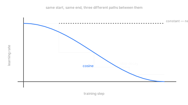
Starting from the same maximum rate, a cosine schedule glides smoothly down to zero while step decay holds flat, then drops in sudden jumps, and a constant rate never decays at all

Why Does This Exist?

Take a 12-layer transformer being trained from scratch on a few million sentence pairs, and pick one fixed learning rate for the entire run. Set it high enough to make fast progress early on, when the random initial weights are far from anything useful, and that same rate is still active a hundred thousand steps later, when the model is close to a good solution and each step should be a small refinement. A rate sized for the beginning keeps kicking the weights past the minimum it's trying to settle into, and the loss curve stops falling smoothly and starts jittering instead — sometimes for the rest of training.

Set the rate low enough to behave well near the end instead, and the first several thousand steps, the ones with the most room to improve, crawl. Neither single number is right for the whole run, because "how big a step should I take" and "how close am I to done" are not questions with the same answer at step 100 and step 100,000.

Think of It Like This

Parking a car

Pulling into a large empty parking lot, you drive at a normal speed to cover the distance quickly — there's nothing to bump into yet. As the parking spot comes into view, you slow down. By the time the car is a foot from the space, you're barely creeping, adjusting the wheel in small increments until it's centered.

Driving at normal speed the entire way, right up to the final foot, means clipping the curb or the car next to you. Creeping at parking speed for the whole approach means the trip across the lot takes ten times longer than it needs to. The right speed depends on how close you are to the target, and it should fall smoothly as that distance shrinks — not stay fixed for the whole approach.

How It Actually Works

The two shapes almost everyone reaches for

Step decay multiplies the learning rate by a fixed factor — often 0.1 or 0.5 — every fixed number of steps or epochs. It's the oldest and simplest schedule: hold a rate flat for a while, drop it, hold the new rate flat, drop it again. The rate is piecewise constant, with sudden jumps at the drop points rather than a gradual slope.

Cosine annealing follows one cycle of a cosine curve from a maximum rate down to (usually) zero, over the whole planned training run:

\eta_t = \eta_{\min} + \tfrac{1}{2}(\eta_{\max} - \eta_{\min})\left(1 + \cos\!\left(\pi \, \tfrac{t}{T}\right)\right)

$\eta_t$ is the rate at step $t$ , $T$ the total number of planned steps, $\eta_{\max}$ and $\eta_{\min}$ the endpoints. Near $t=0$ the cosine curve is nearly flat, so the rate barely moves at first; near $t=T$ it flattens again, easing into zero rather than snapping there. The middle of the run is where it falls fastest. That smooth, no-sudden-jump shape is why cosine schedules produce visibly steadier loss curves than step decay, and why it's the more common default now.

Warmup-stable-decay, the shape large runs actually use

For the biggest training runs — the ones measured in weeks on many GPUs — restarting or adjusting a cosine schedule is expensive, because $T$ has to be fixed in advance and the whole curve is shaped around it. Warmup-stable-decay splits the run into three phases instead: a short warmup ramping up to the peak rate, a long stable phase holding that peak rate flat, and a decay phase at the end easing it down. The stable phase can be extended or cut short without reshaping anything else, which is the flexibility a multi-week run needs and a single cosine curve doesn't give.

What every schedule is doing, underneath the shape

All three exist for the same reason the parking analogy names directly: the learning rate is doing two different jobs at two different points in training, and no single number is well-suited to both. Adam and AdamW already give each parameter its own effective step size from that parameter's gradient history — a schedule is the separate decision of how the global rate multiplying all of that moves over time. The two mechanisms stack: Adam handles per-parameter scale, the schedule handles the overall pace of the run.

Show Me the Code

Cosine annealing and step decay, evaluated at the same five points in an 1,000-step run.

1import numpy as np2
3
4def cosine_lr(step: int, total_steps: int, lr_max: float = 1e-3) -> float:5    progress = step / total_steps6    return 0.5 * lr_max * (1 + np.cos(np.pi * progress))7
8
9def step_decay_lr(step: int, drop_every: int = 250, factor: float = 0.5,10                    lr_max: float = 1e-3) -> float:11    return lr_max * (factor ** (step // drop_every))12
13
14for step in [0, 250, 500, 750, 999]:15    cos_r, step_r = cosine_lr(step, 1000), step_decay_lr(step)16    print(f"step {step:4d}  cosine {cos_r:.6f}  step-decay {step_r:.6f}")17# -> step    0  cosine 0.001000  step-decay 0.00100018# -> step  250  cosine 0.000854  step-decay 0.00100019# -> step  500  cosine 0.000500  step-decay 0.00050020# -> step  750  cosine 0.000146  step-decay 0.00025021# -> step  999  cosine 0.000000  step-decay 0.000125

At step 250, cosine has already started easing down while step decay is still at its starting plateau — the jump doesn't land until the next boundary. That lag is the practical difference between the two shapes, not just their smoothness.

Watch Out For

Picking a schedule before deciding how long training will run

Cosine annealing needs $T$ , the total step count, fixed in its formula before training starts. Extend the run afterward — more data arrived, or the loss hadn't plateaued — and the curve has already reached zero partway through the extension, so every additional step trains at a learning rate near zero and barely moves the weights. Warmup-stable-decay exists specifically to avoid committing to a fixed horizon this early.

Reading a jittery loss curve as an architecture problem

A model trained with step decay shows periodic jumps in the loss curve right at each drop point, and it's tempting to suspect the architecture or the data. Look at the schedule first: a rate drop of 2x or 10x genuinely changes the size of every subsequent step, and a brief transient right after a drop is the schedule working as designed, not a symptom of something broken elsewhere.

The Quick Version

A fixed learning rate is a compromise: too high late in training, too low early on, right for neither.
Step decay holds the rate flat, then drops it by a fixed factor at set intervals — simple, with sudden jumps.
Cosine annealing follows a smooth curve from a maximum rate down to near zero over the whole run.
Warmup-stable-decay splits a run into ramp-up, a long flat plateau, and ramp-down — used on the largest training runs because the plateau length isn't fixed in advance.
A schedule adjusts the shared global rate over time; Adam's per-parameter scaling is a separate mechanism, and the two stack.