Core ML

Loss Functions

Every common loss is the negative log-likelihood of some noise model, so picking one is a claim about how your data got its errors. Choose the claim first.

Squared error keeps curving upward so a single extreme residual dominates the gradient, while absolute error and Huber both grow at a fixed rate once past Huber's threshold

Why Does This Exist?

You're predicting next month's repair bill for each van in a delivery fleet. Most bills land between 200 and 800 dollars. One van in three hundred needs an engine rebuild at 9,000. You minimise squared error because it's the default, and every prediction comes back high — 1,400 dollars quoted for an oil change.

Nothing is broken. Squared error asserts that a residual of 8,000 is ten thousand times more surprising than one of 80, and given that belief, chasing the rebuild is correct.

Every loss in common use is the negative log-likelihood of some noise model. Choosing one is choosing what you believe about how your data got its errors, which turns the list into a decision.

One idea to have in hand: maximum likelihood estimation picks the parameters making the observed data most probable under an assumed distribution. Probabilities multiply and underflow, so take the logarithm and flip its sign.

Think of It Like This

Sliding the pivot under a loaded plank

Ten people stand on a long plank, and you slide a pivot underneath.

Balance it and the pivot lands at the centre of mass: pull grows with distance, so the person at the far end drags the pivot toward them. That's squared error, and the pivot is the mean.

Ignore distance instead. Slide the pivot until five people stand on each side, then stop. The person at the end counts as one, like everyone near the middle. That's absolute error, and the pivot is the median.

Or cap the pull: it grows with distance up to a metre out, then holds flat. Near the pivot it balances, far out it counts. That's Huber.

How It Actually Works

Every loss is a claim about the noise

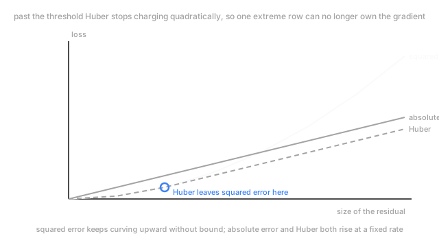
Squared error, $\tfrac{1}{2}(y - \hat{y})^2$ , with $y$ the truth and $\hat{y}$ the prediction. The negative log of a normal density is that plus a constant, so it assumes Gaussian noise of constant variance. Its slope is the residual itself: a row off by 9.0 pushes ninety times as hard as one off by 0.1. Across ten residuals with one at 9.0, that row owns 78 percent of the gradient.

Absolute error, $|y - \hat{y}|$ , is the negative log-likelihood of a Laplace distribution, whose tails are far heavier. Its slope is $+1$ or $-1$ and nothing else, so distance stops buying influence and that row drops to 10 percent. It targets the median, not the mean — here, 0.15 against 0.95.

Huber switches at a threshold $\delta$ (delta): squared inside, absolute outside. It's the negative log-likelihood of a distribution normal in the middle and exponential-tailed beyond, which describes most cost data fairly. You keep the smooth centre and the bounded tail pull. The price is one more number, in the target's units.

Then the losses that price an asymmetry. Quantile loss charges the two sides of the residual differently, so at $\tau = 0.9$ an under-prediction costs nine times an over-prediction — what a parts budget wants. Poisson and Tweedie deviance cover counts and costs piling up at zero with a positive tail. Focal loss is a reweighting, not a noise model: it scales each example's cross-entropy by how badly it's predicted, so a confident majority row barely contributes.

Cross-entropy, and the gradient that made it standard

Classification changes the noise model: there's no residual to be Gaussian about, only a category and a probability over categories. Cross-entropy is the negative log-likelihood of that outcome.

Its gradient is why it won. Take the raw score before squashing, call it $z$ , push it through a sigmoid or softmax for a probability $p$ , then measure against the true label $y$ :

\frac{\partial L}{\partial z} = p - y

Predicted minus actual. No leftover factor, no derivative of the squashing function — the sigmoid's slope cancels against the logarithm's exactly. A confidently wrong prediction gives a gradient near 1 rather than the near-zero one squared error produces on a saturated sigmoid, which is why logistic regression uses this loss.

A loss must be differentiable; a metric needn't be

A loss is what the optimiser minimises, so gradients have to flow through it — backpropagation needs a slope at every step. A metric is what you report, and can be anything.

Accuracy is the clean example. Change a weight by a hair and no prediction crosses its threshold, so the gradient is zero. Change it enough and one prediction flips, and accuracy jumps by a step. Nothing to descend, which is why nothing trains on it — and regression metrics diverge from their losses more often than people expect.

Show Me the Code

Nine ordinary residuals and one engine rebuild. What share of the update does that row ask?

1import numpy as np2
3def gradient_share(loss: str, residuals: np.ndarray, delta: float = 1.0) -> float:4    if loss == "squared":5        g = residuals  # slope of 0.5*r^2, so an extreme row pulls proportionally harder6    elif loss == "absolute":7        g = np.sign(residuals)8    else:9        g = np.clip(residuals, -delta, delta)  # Huber: squared inside, absolute outside10    pull = np.abs(g)11    return float(pull.max() / pull.sum())  # the share of the update one row is asking for12
13repairs = np.array([0.2, -0.4, 0.1, 0.3, -0.2, 0.5, -0.1, 0.4, -0.3, 9.0])  # last one: engine14for name in ("squared", "absolute", "huber"):15    print(f"{name:9s} worst row owns {gradient_share(name, repairs):.1%} of the gradient")16# -> squared   worst row owns 78.3% of the gradient17# -> absolute  worst row owns 10.0% of the gradient18# -> huber     worst row owns 28.6% of the gradient

One row of ten steering four fifths of the update, and nothing in the logs will say so. The loss falls, the curve looks healthy, and the model is fitting one van.

Watch Out For

Squared error on a heavy-tailed target

The tell shows up in one plot: predictions run high across the bulk of the data and low on the extremes. Mean error near zero, median error clearly positive. That's squared error doing what it was asked, with a handful of rows owning the gradient.

Three fixes. Switch to Huber, with $\delta$ near a high percentile of the residuals you'd call ordinary. Or model the logarithm of the target, though back-transforming then predicts a median rather than a mean. Or use Tweedie deviance for costs clustered at zero. What doesn't work is deleting the extreme rows. Those vans exist.

Optimising a loss nobody's decision depends on

Symptom: the training loss improves week over week and the number the team reviews sits still. Every iteration looks like progress in the notebook and none of it lands downstream.

The loss and the decision disagree about what matters. If the output is a ranked shortlist — the ten vans to book in on Monday — then squared error on the predicted bill is optimising something else: it spends capacity on the middle of the distribution, and the middle never reaches the shortlist. A classifier on "will this van land in the worst ten percent" beats a well-fitted regression.

The Quick Version

Every common loss is the negative log-likelihood of a noise model: picking one asserts how your errors arose.
Squared error assumes constant-variance Gaussian noise, targets the mean, and lets one extreme row dominate.
Absolute error assumes heavier tails, charges at a constant rate, and targets the median.
Huber is squared inside a threshold and absolute outside, capping the tail's pull.
Cross-entropy is the classification default, and its gradient on the raw score is predicted minus actual.
Quantile loss prices asymmetry, focal loss down-weights a confidently predicted majority, Tweedie deviance handles counts.
A loss must be differentiable; a metric needn't be, which is why nothing trains on accuracy.