Core ML

Logistic Regression

It classifies, despite the name. A linear score goes in, a sigmoid squeezes it down into a probability, and the log-odds come out straight in the features.

The sigmoid turns an unbounded linear score into a probability between 0 and 1, and the decision boundary sits at the single point where that score is zero and the probability is exactly one half

Why Does This Exist?

You want a yes-or-no answer with a number attached to how sure you are. Not "this subscriber will cancel" but "there's a 78% chance this subscriber cancels next month", because 78% and 51% deserve different phone calls.

The case we'll carry down the page: 40,000 subscribers, one feature each (days since their last login), and last month's outcome, cancelled or stayed.

Try a straight line first. Fit days-since-login against a 0-or-1 label and you get predictions like 1.4 and -0.31, which aren't probabilities, and clipping them hides the real damage: squared error keeps chasing subscribers at 60 idle days who are already correctly classified, so a few far-out points tilt the whole line and ruin the fit where your uncertain subscribers live.

Two words before we go on. Odds restate a probability as a ratio: 0.8 is 4-to-1, four cancellations per stay. Log-odds are the logarithm of that ratio, and the logarithm takes the handcuffs off. Probabilities are trapped in $[0, 1]$ , odds in $[0, \infty)$ , log-odds run across the whole real line — room enough for a straight line.

Which is where the name comes from. Logistic regression really does regress something, linearly. It regresses the log-odds.

Think of It Like This

A tug-of-war where the flag can only move so far

Two teams on a rope. Every feature is a person pulling: their strength is the feature's value times its weight, and the sign of that weight picks their side. Add everyone up and you get the net pull, which can be any number at all, because one team can out-haul the other by an inch or by a landslide.

Now watch the flag tied to the middle of the rope. It can't leave the pit. Even pull, flag on the centre line. One side winning a little, it drifts. One side winning overwhelmingly and it's jammed against the far ditch, where another strong puller joining moves it almost nowhere. Net pull is the linear score, flag position is the probability, centre line is the decision boundary — and that jamming is why extra evidence stops paying once you're already sure.

How It Actually Works

Score, squash, done

Start with a linear score:

z = w^\top x + b

$w$ is one weight per feature, $x$ one subscriber's features, $b$ the intercept. For any subscriber, $z$ is a single unbounded number.

Squash it with the sigmoid, also called the logistic function:

\sigma(z) = \frac{1}{1 + e^{-z}}

$e$ is the usual 2.718. Big positive $z$ drives $e^{-z}$ toward zero and $\sigma(z)$ toward 1. Big negative $z$ blows it up and pushes $\sigma(z)$ toward 0. At $z = 0$ it lands on exactly $0.5$ .

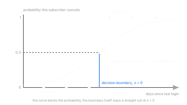
Invert that and you get the claim from the top: $\log \frac{p}{1-p} = z$ , where $p$ is the predicted probability. Log-odds, linear in the features. All the curvature in the diagram happens in the squashing step.

Why squared error is the wrong loss here

Two reasons, and both matter.

Put a sigmoid in the middle and squared error stops being convex in $w$ , growing local dips a gradient method can settle into and never leave. Convexity guarantees one bottom, and you just gave it up for nothing.

Worse, it quits exactly when you need it. Squared error's gradient carries a factor of $\sigma'(z) = \sigma(z)(1 - \sigma(z))$ , which collapses toward zero at both extremes. Predict 0.999 for a subscriber who stayed and you're badly wrong, but that $\sigma'$ factor shrinks the correction to nearly nothing. Learning stalls on your worst cases.

Binary cross-entropy fixes both:

L = -\big[\, y \log p + (1 - y) \log (1 - p) \,\big]

$y$ is the true label, 0 or 1. Predict 0.999 when the truth is 0 and $-\log(0.001)$ charges you about 6.9, with the penalty running to infinity as confidence in the wrong answer grows. The algebra is kind too: the $\sigma'$ term cancels against the log, leaving a gradient of $(p - y)\,x$ . Prediction minus truth, times the input.

Reading the coefficients

Because $z$ is log-odds, a one-unit rise in feature $j$ adds $w_j$ to the log-odds, which multiplies the odds by $e^{w_j}$ . A weight of 1.16 triples the odds. It does not mean the probability rises by a fixed amount: 0.02 to 0.06 and 0.5 to 0.75 are both a tripling.

The boundary is a hyperplane sitting where $z = 0$ . Flat. Straight. The sigmoid bends the probability surface, not the boundary, so classes a straight cut can't separate need interaction features or a different model.

Show Me the Code

Fit it by hand, then read the coefficient as an odds multiplier.

1import numpy as np2
3def sigmoid(z: np.ndarray) -> np.ndarray:4    return 1.0 / (1.0 + np.exp(-z))5
6def fit(X: np.ndarray, y: np.ndarray, lr: float = 0.5, steps: int = 3000) -> np.ndarray:7    w = np.zeros(X.shape[1])8    for _ in range(steps):9        # cross-entropy's whole payoff: the gradient is just (p - y) x, no sigmoid' factor10        w -= lr * X.T @ (sigmoid(X @ w) - y) / len(y)11    return w12
13rng = np.random.default_rng(0)14idle = rng.uniform(0.0, 60.0, 4000)                     # days since last login15left = (rng.random(4000) < sigmoid(0.12 * idle - 3.6)).astype(float)16X = np.column_stack([np.ones_like(idle), idle / 10.0])  # one unit = 10 idle days17w = fit(X, left)18print(f"odds x{np.exp(w[1]):.2f} per 10 idle days, 50% at {-10 * w[0] / w[1]:.0f} days")19# -> odds x3.19 per 10 idle days, 50% at 30 days

Every ten idle days roughly triples the odds of cancelling, and the boundary lands at 30 days, which is where the truth was planted.

Watch Out For

Perfectly separable data sends the weights to infinity

Add a feature that separates your classes cleanly and the training loss falls, keeps falling, and never settles. The symptom is coefficients in the hundreds after a long run and the thousands after a longer one, with standard errors that are enormous or refuse to compute. Nothing is broken. If a boundary separates the data perfectly, scaling $w$ up sharpens every prediction, so the likelihood improves without limit and no finite optimum exists.

More iterations make it worse. The fix is a penalty on the weights, and Ridge-style shrinkage is what most libraries quietly apply by default. Go looking first, though, because near-perfect separation in production data is usually leakage rather than luck: a cancellation-survey timestamp that only exists for people who cancelled separates your classes beautifully and predicts nothing.

Treating the sigmoid output as a calibrated probability

Unregularised logistic regression on a representative sample is genuinely close to calibrated, which is why it survives in credit and insurance work where the number itself gets used. But calibration belongs to the data you fitted on, not to the sigmoid. Reweight the classes to fight imbalance or downsample the majority, and your intercept now describes a population that doesn't exist. A predicted 0.30 might mean 0.04 in the wild.

The symptom is quiet: rankings stay fine, so accuracy and AUC look untouched while every expected-value calculation downstream is inflated. Bucket your predictions, compare each bucket's mean prediction to its observed rate, then correct the intercept or fit a calibration map — probability calibration covers both.

The Quick Version

It's a classifier. The "regression" is honest about one thing: log-odds are linear in the features.
Three pieces. A linear score $z$ , a sigmoid turning it into a probability, binary cross-entropy as the loss.
Squared error is wrong twice: non-convex through the sigmoid, and its gradient dies when the model is confidently wrong.
Cross-entropy's gradient is $(p - y)\,x$ . Prediction minus truth, times the input.
The boundary is a flat hyperplane at $z = 0$ . Curvature lives in the probability, not the boundary.
One unit of feature $j$ multiplies the odds by $e^{w_j}$ , and never shifts the probability by a fixed amount.
Perfect separability has no finite solution. Regularise; don't iterate harder.