Generalized Linear Models
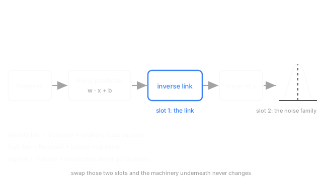
Least squares and logistic regression are the same machine with two settings, a link function and a noise family. Swap them and count data starts working.
Why Does This Exist?
Your helpdesk logs support tickets. Some days none, most days a handful, one memorable Tuesday forty-one. You have the promotional emails marketing sent that morning, and you want to know what each extra email costs you in tickets.
Reach for least squares and it hands you an answer. Ask what happens on a day with no promos and it predicts negative 4.8 tickets. Not rounded up to zero, not flagged. A number that cannot exist, stated with a straight face. And the negative is only half the trouble, because least squares also assumes constant spread, while quiet days vary by two or three tickets and busy days by fifteen.
Now look at what you already know. Linear regression predicts a mean directly and assumes bell-shaped noise. Logistic regression runs the same linear score through a sigmoid and assumes coin-flip noise. Those look like two models. They're one model with two dials set differently, and once you can see the dials you stop inventing a new loss every time your target changes shape. Both are fitted by maximum likelihood: pick the parameters that make the data you actually observed as unsurprising as possible.
Think of It Like This
One camera body, two swappable parts
The body never changes. Same shutter, same mount, same mechanism turning what's in front of it into a picture. That's your linear predictor: features in, one weighted sum out.
The lens changes the geometry. A wide lens and a long lens point at the same scene and put it on the frame differently, and neither alters the body. That's the link function, deciding how the weighted sum maps onto the thing you're predicting. A log lens can only produce positive output, exactly what you want when the thing is a count of tickets.
The film changes the grain. That's the noise family: how much spread to expect around the value you predicted, and whether that spread grows with it. Wrong lens, impossible pictures. Wrong film, right picture with the wrong confidence in it. The body is fine either way, which is why swapping those two parts is the whole skill.
How It Actually Works
Three parts, two of them choices
The first is the linear predictor, unchanged from least squares:
(eta) is a plain real number, one per row. holds the weights, one day's features, the intercept.
The second is the link function , connecting to , the expected value of the response for that row:
The inverse link is what runs at prediction time, and it's where impossible values get ruled out. Pick and its inverse is , positive for every that ever existed. No negative ticket counts, structurally, not by clipping.
The third is the distribution family around : Gaussian, Bernoulli, Poisson, Gamma. All belong to the exponential dispersion family, whose shape forces a mean-variance relationship out for free. Fix the family and you've fixed how the spread grows with the mean.
The three settings you'll actually use
Identity link, Gaussian family. , constant variance, and maximising the likelihood reduces exactly to minimising squared error. That's ordinary least squares wearing a longer name.
Logit link, Bernoulli family. is a probability, , and the variance peaks at 0.5 and vanishes at both ends. That's logistic regression.
Log link, Poisson family. , and the variance equals the mean. This is the setting nobody teaches and everybody needs: tickets per day, clicks per hour, defects per batch. It answers the negative-4.8 problem and costs one keyword in most libraries.
When Poisson isn't enough
Poisson makes a testable promise: variance equals mean. Real count data usually breaks it. Days cluster, one outage spawns thirty tickets, an unmodelled feature shifts the whole rate, and the observed spread lands above the mean. That's overdispersion, and the damage is specific: coefficients stay roughly right while standard errors come out too small, so you report a significant effect that isn't there.
Check it on the residuals, not the raw column, since a raw variance-to-mean ratio of 10 mostly reflects the features doing their job. Conditioned on the fit, that ratio sits near 1 if Poisson holds. If it's 2, the honest fix is the negative binomial family, which is Poisson with a second parameter for exactly this slack.
Code
Fit Poisson with Newton steps, then let least squares embarrass itself on the same 500 days.
import numpy as np
def fit_poisson(X: np.ndarray, y: np.ndarray, steps: int = 50) -> np.ndarray: w = np.zeros(X.shape[1]) for _ in range(steps): mu = np.exp(X @ w) # the inverse log link, so every fitted mean stays positive w += np.linalg.solve(X.T @ (X * mu[:, None]), X.T @ (y - mu)) return w
rng = np.random.default_rng(1)emails = rng.uniform(0.0, 3.0, 500) # promo emails sent that dayX = np.column_stack([np.ones_like(emails), emails])tickets = rng.poisson(np.exp(0.4 + 1.1 * emails)) # support tickets that dayw = fit_poisson(X, tickets)ols = np.linalg.lstsq(X, tickets.astype(float), rcond=None)[0]print(f"poisson: x{np.exp(w[1]):.2f} tickets per extra email, {np.exp(w[0]):.1f} at zero")print(f"ols at zero emails: {ols[0]:.1f} tickets")# -> poisson: x2.99 tickets per extra email, 1.5 at zero# -> ols at zero emails: -4.8 ticketsEach extra email triples the ticket rate, and a quiet day sits at 1.5. The straight line predicts minus 4.8.
Watch Out For
Fitting least squares to a count or a rate
The symptom is easy to spot once you look: negative predictions at the low end of the range, and residuals fanning out like a wedge as the fitted value grows. Both come from the same source. The identity link has nothing stopping it below zero, and the Gaussian family insists the spread is constant when counts make it grow with the mean.
The temptation is to patch it with and fit least squares to that. Popular, fast, and it changes the question. You're now modelling the mean of the log rather than the log of the mean, so exponentiating back gives you something closer to a median, biased low. It also forces you to invent a constant for the zeros, and your answer moves depending on whether you picked 1 or 0.5.
Reading log-link coefficients as if they were additive
A coefficient of 0.3 under a log link does not mean "0.3 more tickets". It means , so 35% more tickets, multiplicatively, from whatever the baseline happened to be. On a quiet day that's half a ticket. On the Tuesday you got forty-one, it's fourteen.
This one survives review, because 0.3 sounds modest and the summary table looks like a least-squares table. Exponentiate every coefficient before it leaves your notebook and label the column as a rate ratio. The intercept is on the same scale: is the rate when every feature is zero, which only means something if zero is a state your data contains.
The Quick Version
- Three parts: a linear predictor, a link tying it to the mean of the response, a distribution family for the noise.
- The link and the family are the two settings. Everything else is shared machinery, fitted by maximum likelihood.
- Identity + Gaussian is least squares. Logit + Bernoulli is logistic regression. Log + Poisson is count regression.
- Use a log link the moment your target can't be negative. Impossible predictions become unreachable.
- Overdispersion leaves coefficients right and standard errors too small. Negative binomial fixes it.
- Log-link coefficients multiply. , never an additive shift.