Core ML

Ridge Regression

Add a penalty on coefficient size and the bias-variance tradeoff becomes a dial you turn: accept a little bias on purpose, buy a much bigger drop in variance.

Every coefficient slides smoothly toward zero as the penalty grows and none of them ever arrives, so held-out error is what picks the point on the path you ship

Why Does This Exist?

Thirty wheat fields. Forty sensor readings each, one yield number per field. Fit plain least squares through that and two soil-moisture probes buried three metres apart — probes that agreed all season to within a rounding error — come back with coefficients of $+207$ and $-205$ .

Nothing about wheat says that. The fit noticed that probe 1 minus probe 2 is a nearly empty column of measurement noise, and that multiplying nearly nothing by two hundred threads the thirty training points a fraction closer. Then somebody recalibrates a probe, the two giants stop cancelling, and held-out error goes from 0.37 to 17.6.

One term fixes it. Least squares picks the coefficients — one number per sensor, saying how much predicted yield moves per unit of that reading — that make the sum of squared misses smallest. That objective has no opinion about how big those numbers get. Ridge hands it one.

Think of It Like This

Springs pulling every dial back to its zero mark

You're tuning forty dials on a mixing desk to match a recording, and plenty of settings match it about equally well.

Now attach a spring from each dial to its zero mark, and make the spring's cost grow with the square of how far you've pulled. The second centimetre costs three times the first. Two things follow.

Cancelling extremes stop being affordable. One dial at $+207$ and its neighbour at $-205$ costs about 85,000 in spring energy; splitting the same job as $+0.9$ and $+0.9$ costs 1.6. The desk starts preferring the flat, boring setting, which is also the one that survives a recalibrated probe.

And no dial ever snaps onto zero. A spring's pull weakens as the dial closes in, and at zero displacement there's no pull left, so there's never a final tug to shut the gap. Dials get arbitrarily close and park there.

How It Actually Works

The same squared-error objective, with one term bolted on:

\sum_{i=1}^{n} \big(y_i - x_i^\top w\big)^2 + \lambda \lVert w \rVert_2^2

Here $y_i$ is field $i$ 's actual yield, $x_i$ its row of sensor readings, and $w$ the vector of coefficients you're solving for. The term $\lVert w \rVert_2^2$ is the sum of the squared coefficients, the squared L2 norm. And $\lambda$ is the dial: at zero you have plain least squares back, and as it grows every coefficient gets squeezed.

The ridge running down the diagonal

Set the derivative to zero and the answer is closed form, same as ever:

w = \big(X^\top X + \lambda I\big)^{-1} X^\top y

$X$ is the whole 30-by-40 table and $I$ is the identity matrix, ones down the diagonal and zeros elsewhere. So $\lambda I$ adds $\lambda$ to each diagonal entry of $X^\top X$ and touches nothing else. A ridge, running down the diagonal. That's where the name comes from.

It's also the entire numerical argument. With forty columns and thirty rows, $X^\top X$ is singular — least squares has no unique answer at all. Adding $\lambda I$ lifts every eigenvalue by exactly $\lambda$ , all of them turn strictly positive, and the matrix inverts. Two near-identical probes are the same disease in milder form: an eigenvalue near zero rather than at it.

Standardise first, and leave the intercept alone

The penalty charges by coefficient magnitude, and magnitude depends on the unit underneath it. Nitrogen in parts per million sits around 200, so its coefficient is small. Soil moisture as a fraction sits between 0 and 1, so to shift yield by the same amount its coefficient must be hundreds of times larger — and the penalty, squaring that, charges it tens of thousands of times more. Same physics, opposite treatment, decided by whoever labelled the column.

So standardise every column first: subtract its mean, divide by its standard deviation. Skip it and $\lambda$ isn't a modelling choice, it's a statement about your measuring units.

The intercept stays out of the penalty. It's the predicted yield when every sensor sits at its average, and shrinking it toward zero asserts that a thoroughly average field grows nothing. Every implementation excludes it.

What the path costs you

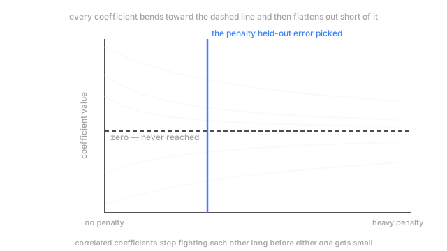
Turn $\lambda$ up and each coefficient traces a smooth curve toward zero without landing on it — that's the diagram, and the smoothness is the spring losing its grip. At $\lambda = 10$ the two probes come back at 0.7 each when a fair split of the truth would be 1.0 apiece, so the model runs systematically low. That's bias, bought on purpose.

The trade pays only if variance falls further than bias rises, and there's one way to find out: fit at each $\lambda$ on training folds, score on held-out folds, keep the best. Cross-validation isn't a refinement here — $\lambda$ has no correct value derivable from data you've already fitted.

Show Me the Code

Eight columns instead of forty, so the numbers fit on a line.

1import numpy as np2
3
4def ridge(X: np.ndarray, y: np.ndarray, lam: float) -> np.ndarray:5    # lam on the diagonal lifts every eigenvalue of X.T @ X, so this still solves when6    # two columns are near-identical and plain least squares is effectively singular7    return np.linalg.solve(X.T @ X + lam * np.eye(X.shape[1]), X.T @ y)8
9
10def season(n: int, gap: float, rng: np.random.Generator) -> tuple[np.ndarray, np.ndarray]:11    X = rng.normal(size=(n, 8))12    X[:, 1] = X[:, 0] + rng.normal(0.0, gap, n)  # probe 2 sits three metres from probe 113    return X, X[:, 0] * 2.0 + rng.normal(0.0, 0.5, n)14
15
16rng = np.random.default_rng(1)17Xtr, ytr = season(30, 0.001, rng)18Xte, yte = season(5000, 0.02, rng)  # next season the two probes drift apart19for lam in (0.0, 0.1, 10.0):20    w = ridge(Xtr, ytr, lam)21    print(f"{lam:5.2f}  probes {w[0]:7.1f} {w[1]:8.1f}   held-out MSE {np.mean((yte - Xte @ w) ** 2):6.2f}")22    # ->  0.00  probes   207.0   -205.2   held-out MSE  17.6423    # ->  0.10  probes     0.9      0.9   held-out MSE   0.3724    # -> 10.00  probes     0.7      0.7   held-out MSE   0.63

A penalty of 0.1 cuts held-out error by a factor of forty-eight and makes the probes agree. A penalty of 10 over-shrinks and hands some of that back. Nothing but held-out error was going to find the value in between.

Watch Out For

Fitting on raw units and then calling lambda a hyperparameter

The symptom: your chosen $\lambda$ moves three orders of magnitude when a colleague switches one column from grams to kilograms, and the surviving coefficients reshuffle with it. Nothing about the soil changed. The penalty was measuring your unit choices, and cross-validation dutifully optimised over them.

Standardise, and do it inside each fold rather than once over the whole table. Taking a column's mean and standard deviation across all rows before splitting hands held-out statistics to the training set — data leakage of the small, believable kind that lifts every score a little. A scikit-learn Pipeline wires this correctly; feature scaling has the mechanics.

Tuning lambda on the data you then report the score from

Best cross-validated error 0.31, production error 0.48. Every project, same direction. You searched forty values of $\lambda$ and reported the winner, and the winner won partly on merit and partly on which rows landed in which fold. Reporting the maximum of a noisy search keeps the luck and discards the evidence.

Split a test set off before you tune anything and score it once. If the dataset is too small to spare, use nested cross-validation: an inner loop picks $\lambda$ , an outer loop scores the whole pick-then-fit procedure. The number you publish comes from rows no hyperparameter ever saw — see train, validation and test splits.

The Quick Version

Ridge adds $\lambda \lVert w \rVert_2^2$ to squared error. One term, one number to tune.
The closed form gains $\lambda I$ on the diagonal — the name and the reason it works. Every eigenvalue lifts by $\lambda$ , so the matrix inverts even with more features than rows.
Coefficients shrink smoothly toward zero and never reach it, because a squared penalty's pull vanishes as the coefficient does. Ridge shrinks; it doesn't select.
Correlated features get the load split rather than fought over.
Standardise first, or $\lambda$ penalises whichever feature you measured in small units. Never penalise the intercept.
You're buying variance reduction with bias, deliberately. Held-out error is the only judge — and it has to come from rows that had no say in choosing $\lambda$ .