Core ML

Model Pruning

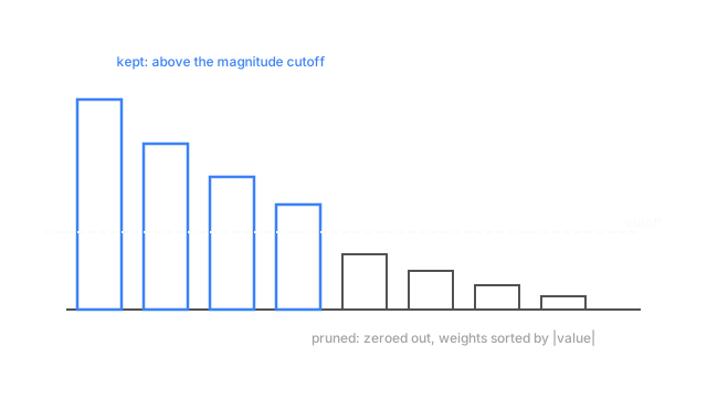
Most of a trained network's weights are small enough to zero out with almost no accuracy loss, so pruning finds and removes exactly those, leaving it sparse.

Weights sorted by magnitude form a curve; a threshold line marks the cutoff, and every bar below it gets zeroed out while the tallest bars survive untouched

Why Does This Exist?

A voice assistant's wake-word detector runs on a smart speaker's tiny onboard chip, always listening, always constrained to a strict power and memory budget. The best-performing model anyone trained for this task has 8 million parameters. The chip has room for roughly 500,000.

Training a smaller network from scratch is the obvious answer, and it underperforms — a network designed to be that small from the start misses accuracy the 8-million-parameter one gets almost for free, because it never had the extra capacity to explore during training. But once the large network is trained, something becomes visible that wasn't visible during training: a large share of its weights are close to zero. They contributed almost nothing to any prediction, they just weren't costing anything to keep around either — until now, when every parameter costs real memory on a chip that doesn't have much.

Model pruning removes those near-zero weights directly from an already-trained network, rather than training a smaller one from scratch.

Think of It Like This

Thinning a hedge that's already grown

A hedge has grown thick over a season — most of it useful, holding the overall shape, but a fair number of thin, weak branches tangled inside that aren't holding anything up. A gardener doesn't replant the hedge smaller from a fresh cutting. They go through the grown hedge and cut out specifically the thin, weak branches, leaving the structural ones untouched.

The hedge afterward looks almost the same from the outside — same shape, same coverage — but it's lighter, and most of what made it strong is exactly what's still there. Pruning is that same cut: go through an already-grown network, remove the connections that were barely holding anything up, and keep the ones that were.

How It Actually Works

Ranking weights by magnitude

The simplest and still most common pruning method is magnitude pruning: after training, take every weight's absolute value, sort them, and zero out the smallest fraction — say, the bottom 90%. The reasoning is direct: a weight near zero contributes almost nothing to the layer's output no matter what input it sees, so removing it changes the network's behavior the least of any weight you could remove. It's a rough proxy for importance, not a perfect one, but it's cheap to compute and it works well enough to be the default starting point.

Unstructured versus structured pruning

Unstructured pruning zeros out individual weights wherever they fall in the magnitude ranking, producing a sparse matrix with an irregular scatter of zeros. It gets the best accuracy-for-a-given-sparsity tradeoff, but ordinary hardware doesn't skip multiplying by a zero any faster than a nonzero — the matrix is still dense in memory unless the software stack specifically supports sparse operations, which most consumer chips don't.

Structured pruning removes whole rows, columns, or channels at once — an entire neuron, an entire convolutional filter. This shrinks the actual matrix dimensions, so hardware benefits immediately, no sparse-matrix support required. The cost is a coarser cut: removing a whole channel throws away whatever small useful signal was mixed in alongside the near-zero weights around it, so structured pruning at equal sparsity typically costs more accuracy.

Fine-tuning after the cut, and why it's necessary

Zeroing out 90% of a network's weights in one pass and evaluating it immediately usually produces a network that's noticeably worse — the remaining weights were trained assuming their now-deleted neighbors were still contributing. Fine-tuning after pruning, continuing training for a modest number of steps with the pruned weights held at zero, lets the surviving weights adjust to their new context. This recovery step isn't optional in practice: skipping it systematically understates how much sparsity a network can tolerate.

The lottery ticket hypothesis

A 2019 finding complicated the "prune what's already trained" story: inside a large randomly-initialized network, there often exists a much smaller subnetwork that, if trained by itself from that same random starting point, reaches comparable accuracy to the full network. Ordinary pruning — train large, then prune — is one way of finding that subnetwork after the fact, but the hypothesis suggests its capability was latent in the initialization, not something training created and pruning merely revealed. That reframes pruning as searching for a lucky, sparse subnetwork already present at the start.

Show Me the Code

Sorting weights by magnitude and checking how much of the network's total squared magnitude survives at different sparsity levels.

1import numpy as np2
3
4def prune_by_magnitude(w: np.ndarray, sparsity: float) -> np.ndarray:5    """Zero out the smallest `sparsity` fraction of weights by absolute value."""6    k = int(round(sparsity * w.size))7    if k == 0:8        return w.copy()9    threshold = np.sort(np.abs(w).ravel())[k - 1]10    return np.where(np.abs(w) > threshold, w, 0.0)11
12
13rng = np.random.default_rng(4)14w = rng.normal(0, 1, size=(64, 64))15total_energy = float((w ** 2).sum())16for sparsity in (0.5, 0.9, 0.98):17    pruned = prune_by_magnitude(w, sparsity)18    kept_energy = float((pruned ** 2).sum())19    nonzero = int((pruned != 0).sum())20    print(f"sparsity {sparsity:.0%}: kept {nonzero}/{w.size} weights, retains {kept_energy / total_energy:.1%} of magnitude energy")21# -> sparsity 50%: kept 2048/4096 weights, retains 92.8% of magnitude energy22# -> sparsity 90%: kept 410/4096 weights, retains 44.0% of magnitude energy23# -> sparsity 98%: kept 82/4096 weights, retains 14.8% of magnitude energy

Removing half the weights only gives up 7.2% of the total magnitude energy, because the smallest weights were contributing almost nothing to begin with. Push to 98% sparsity and the picture changes — you're now cutting into weights that were carrying real signal, which is exactly why fine-tuning becomes necessary past a certain sparsity level, not optional.

Watch Out For

Evaluating a pruned network without fine-tuning it

Zeroing out weights and measuring accuracy immediately, with no retraining step, systematically understates how much sparsity a network can tolerate — the surviving weights haven't had a chance to adjust to their now-sparser neighborhood. A pruning comparison that skips fine-tuning will make every method look worse than it actually performs in practice, and can lead to under-pruning a network that could have gone considerably sparser.

Choosing unstructured pruning for a deployment target that can't exploit sparsity

Unstructured pruning gets the best accuracy at a given sparsity level on paper, but if the deployment hardware has no sparse-matrix support, the "pruned" network still occupies the same memory and runs at the same speed as the dense one — none of the promised savings materialize. Check what the target hardware or inference runtime actually supports before choosing between structured and unstructured pruning; the better number on a benchmark table is irrelevant if it can't be realized on the chip you're shipping to.

The Quick Version

Magnitude pruning zeros out the smallest-magnitude weights in an already-trained network, on the reasoning that they contribute the least to its output.
Unstructured pruning gets better accuracy per unit of sparsity but needs sparse-aware hardware or software to realize any actual speedup; structured pruning removes whole channels and works on ordinary hardware immediately.
Fine-tuning after pruning is necessary in practice, not optional — the surviving weights need to adjust to their pruned neighborhood.
The lottery ticket hypothesis suggests small, well-performing subnetworks are often already latent in a large network's random initialization, reframing pruning as a search rather than pure compression.