Core ML

Patch Embeddings

Patch embeddings flatten each fixed-size image patch into a vector, then project it once into a token dimension a transformer block can actually read.

One highlighted patch is cut from the image grid, flattened into a raw pixel vector, and projected through one learned matrix into a token vector the model can read

Why Does This Exist?

Vision Transformers need their input as a sequence of token vectors, because that's what self-attention operates over. An image, as it exists on disk, is none of that — it's a 2D (or 3D, counting color channels) grid of pixel intensities, with no notion of "tokens" anywhere in it. Something has to sit between the raw pixel grid and the first attention layer, converting one representation into the other, and that conversion has to be learned rather than hand-designed, so the model can decide for itself what's worth keeping from each patch.

Patch embeddings are that boundary layer. The wall they solve is narrow but load-bearing: without a defined way to turn a patch of pixels into a fixed-length vector, "run a transformer on an image" isn't a well-formed sentence. Get this step wrong — the wrong patch size, a missing normalization, an unlearned projection — and every layer downstream is attending over garbage, no matter how well-designed the rest of the architecture is.

Think of It Like This

Scanning a photo strip into one barcode per frame

Picture a photo booth strip: four small square photos, side by side. Now imagine a scanner that doesn't try to understand each photo — it just reads every pixel in one square, left to right, top to bottom, and produces one long number for each pixel it saw. That's flattening: a mechanical, lossless unrolling of a 2D square into a 1D list, no interpretation involved yet.

Then a second machine takes that long list of raw numbers and boils it down to a much shorter, denser code — a barcode standing in for "whatever mattered about that patch." That compression step is learned: the machine was trained to produce codes that make later stages' jobs easier, not to preserve every pixel faithfully. Patch embedding is exactly these two steps, back to back: unroll the patch, then compress it into a code the rest of the pipeline can use.

How It Actually Works

Slice the image into fixed, non-overlapping squares

Divide the input image into a grid of patches of a fixed size — 16×16 pixels is the standard choice for a 224×224 image, giving a 14×14 grid, 196 patches total. The patches don't overlap and don't skip any pixels; every pixel in the image belongs to exactly one patch. Patch size is a real design choice with a real tradeoff: smaller patches mean a longer sequence and finer spatial resolution, at the cost of more tokens for self-attention to process, which matters because attention cost grows with the square of sequence length.

Flatten each patch into a raw pixel vector

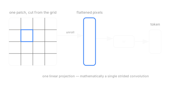
Each patch, still just a grid of numbers, gets unrolled into a single 1D vector by concatenating its rows (or columns) end to end, across all color channels. A 16×16 patch with 3 color channels becomes a vector of length 16 × 16 × 3 = 768 — no computation happens here, just a reshape. This is the step the diagram's middle box represents: the highlighted square from the grid, laid out as one long thin strip of numbers.

Project into the model's embedding dimension

That flattened vector is far too large and far too raw to feed a transformer directly, so one learned linear layer projects it down (or occasionally up) to whatever embedding dimension the model uses internally — commonly 768 or 1024, independent of the patch's own flattened size. This single matrix multiply is the only learned operation patch embedding performs, and it's shared across every patch in every image: the same projection matrix processes patch 1 and patch 196 identically, which is exactly the translation-equivariance property patches inherit from convolution's shared-kernel design.

Why this is, mathematically, one strided convolution

Slicing an image into non-overlapping patches and applying the same linear projection to each one is exactly what a convolution with a kernel size and stride both equal to the patch size computes — a single convolutional layer, with no padding and no overlap, sweeping across the image once. It's worth naming explicitly because it clarifies what's actually novel about a Vision Transformer: not the input layer, which is one ordinary strided convolution, but everything after it, which drops convolution entirely in favor of self-attention.

Show Me the Code

Flattening a small synthetic image into patches and projecting them, tracing the exact shapes at each step.

1import numpy as np2
3
4def patchify(image: np.ndarray, patch_size: int) -> np.ndarray:5    h, w, c = image.shape6    grid = h // patch_size7    patches = image.reshape(grid, patch_size, grid, patch_size, c)8    patches = patches.transpose(0, 2, 1, 3, 4)9    return patches.reshape(grid * grid, patch_size * patch_size * c)10
11
12rng = np.random.default_rng(0)13image = rng.normal(size=(8, 8, 3))                       # tiny 8x8 RGB image14patches = patchify(image, patch_size=4)15print(patches.shape)   # -> (4, 48) -- 4 patches (2x2 grid), each 4*4*3 pixels flattened16
17embed_dim = 618projection = rng.normal(scale=0.2, size=(patches.shape[1], embed_dim))19tokens = patches @ projection20print(tokens.shape)    # -> (4, 6) -- one 6-dimensional token per patch

The projection matrix's shape, (48, 6), is fixed once and reused for every patch — the same matrix that processes patch 0 processes patch 3, which is why tokens.shape[0] matches the patch count exactly, not some smaller reduced number.

Watch Out For

Picking a patch size without weighing the sequence-length cost

A smaller patch size gives finer spatial detail but multiplies the number of tokens self-attention has to process — halving the patch size quadruples the patch count, and full self-attention's cost grows roughly with the square of that count. Choosing patch size purely for resolution, without checking what it does to the resulting sequence length and attention cost, is a common way to make training or inference far more expensive than intended.

Treating patch embedding as convolution and expecting convolution's other benefits

Patch embedding is mathematically one strided convolution, but it's a single layer applied once, not a stack of convolutions building up a hierarchy of receptive fields the way a CNN does. Assuming it inherits a CNN's multi-scale feature hierarchy just because the first step resembles convolution is a mistake — everything after this one layer is self-attention, with none of a CNN's depth-wise structure, unless the architecture is specifically a hierarchical design.

The Quick Version

Patch embedding cuts an image into fixed, non-overlapping squares, flattens each into a raw pixel vector, then projects it with one shared learned matrix into the model's embedding dimension.
Flattening is a reshape with no computation; the projection matrix is the only learned part, and it's the same matrix for every patch.
The whole operation is mathematically equivalent to a single convolution with kernel size and stride equal to the patch size.
Patch size trades spatial resolution against sequence length, and attention cost scales with the square of that length.
Position information is not part of patch embedding itself — it has to be added separately, since flattening erases spatial layout.