Core ML

Perceptron

One neuron learning a boundary from its own mistakes and nothing else. It halts the instant nothing is wrong, and loops forever when no straight line exists.

Why Does This Exist?

Two pressure mats sit in a warehouse doorway, one inside and one outside. You want an alert when exactly one is pressed: somebody standing in the doorway rather than walking through. Four situations, two worth an alert. Keep those mats in mind, they're going to break something.

Frank Rosenblatt published the perceptron in 1958 and had it in hardware at Cornell within two years: 400 photocells wired to potentiometers that physically turned themselves whenever the machine got an answer wrong. Guess, and when you're wrong, lean the boundary toward what you missed. No loss function, no calculus, no probability. It's the smallest thing anyone calls a neural network, and the wall it hit is why deep learning exists.

One piece of notation. $w^\top x$ is the dot product: multiply matching entries of two vectors and add the results. It measures how much of $x$ points along $w$ , so its sign tells you which side of a flat boundary you're on. That sign is the whole perceptron.

Think of It Like This

A ruler laid across a table of beans

Black beans and white beans scattered on a table. Lay a ruler down so the black ones end up on one side and the white ones on the other. Slide it, pivot it, never bend it.

The procedure is blunt. Point at each bean and say which side you think it's on. Right, do nothing. Wrong, shove the ruler toward the bean you missed. Once every bean is on the correct side nothing triggers a shove, so the ruler stops dead, wherever it happens to be, often lying almost against a bean it barely got right.

Now spill the beans into the four corners of a square, black on one diagonal, white on the other. You can't lay the ruler down, and shoving won't help, because the ruler is straight and the pattern isn't.

How It Actually Works

The rule, in full

Prediction is a sign:

\hat{y} = \operatorname{sign}(w^\top x + b)

$w$ holds one weight per input, $x$ is the current example, $b$ is the bias letting the boundary sit somewhere other than the origin. Labels are written $+1$ and $-1$ rather than 1 and 0, which is the trick that makes the next line short.

Walk the examples. When $\hat{y} = y$ , change nothing. When you get one wrong:

w \leftarrow w + y\,x, \qquad b \leftarrow b + y

Add the input to the weights if you should have said $+1$ , subtract it if you should have said $-1$ . Geometrically, $w$ rotates toward the example you missed, pushing the boundary past it. The update is sized by the input, not by how wrong you were, so a near-miss and a catastrophe get identical treatment.

It provably stops, with one enormous condition

Novikoff proved in 1962 that the number of updates is bounded by

\left(\frac{R}{\gamma}\right)^{2}

$R$ is the length of the longest example vector and $\gamma$ (gamma) is the margin, the distance from the best possible boundary to the nearest point. No dependence on how many examples, or how many features.

Guaranteed if the data is linearly separable. If it isn't, $\gamma$ doesn't exist, the bound says nothing, and the loop runs until you stop it. The weights keep moving, the mistake count bounces without trending, and you can't tell "one more pass" from "never". That's the default case, because real data is almost never separable.

The XOR wall, and what climbing it cost

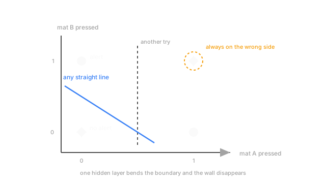
Back to the mats. Encode them as 0 or 1: $(0,0)$ and $(1,1)$ mean no alert, $(0,1)$ and $(1,0)$ mean alert. The alerts sit on one diagonal of a square with the quiet cases on the other. This is exclusive-or, and the diagram shows it — every straight line strands at least one point.

Minsky and Papert made this precise in 1969 and the field stalled on it for over a decade. The fix is short: put a layer of perceptrons in between, let them build new coordinates, and the boundary in the original space can bend. That's the multi-layer perceptron, and two hidden units do it.

The bill came with it. The learning rule works only because it never differentiates anything. Stack layers and you need to know how an inner weight affects the final answer, and the step function's derivative is zero everywhere it exists and undefined at the boundary itself. Nothing to descend. So the step went, replaced by smooth activations, and mistake-driven nudging gave way to gradient descent and backpropagation.

Show Me the Code

The same twelve lines on both mat problems. One terminates; the other can't.

1import numpy as np2
3def train(X: np.ndarray, y: np.ndarray, epochs: int = 100) -> tuple[np.ndarray, int]:4    w = np.zeros(X.shape[1])5    for epoch in range(epochs):6        wrong = 07        for xi, yi in zip(X, y):8            if yi * (w @ xi) <= 0.0:  # a mistake, or sitting exactly on the boundary9                w += yi * xi10                wrong += 111        if wrong == 0:12            return w, epoch  # no point is misclassified, so no update can ever fire again13    return w, epochs  # the cap is the only thing that stops a non-separable run14
15mats = np.array([[1.0, 0, 0], [1, 0, 1], [1, 1, 0], [1, 1, 1]])  # leading 1 is the bias16print(train(mats, np.array([-1.0, -1, -1, 1]))[1], "epochs: alert when both mats press")17print(train(mats, np.array([-1.0, 1, 1, -1]))[1], "epochs: alert when exactly one presses")18# -> 8 epochs: alert when both mats press19# -> 100 epochs: alert when exactly one presses

"Both mats" is separable, so pass 8 sweeps all four points without an update and the function returns. "Exactly one" burns all 100 and returns the cap. Raise the cap to a million; it returns a million.

Watch Out For

Running the update rule on data that isn't separable

The symptom is a loop that finishes because it ran out of epochs, with final weights that are whatever the last mistake left behind. Not the best boundary found along the way, not an average. Weights from one arbitrary moment in an oscillation, and they can be worse than what the loop held fifty passes earlier.

Two guards, both cheap. Cap the epochs and treat hitting the cap as a result, not as completion. Then track the mistake count each pass and keep the weights from the best one, which is the pocket perceptron and takes four lines. Better still, notice what you're doing: on messy data, logistic regression minimises a convex loss with a finite answer.

Assuming the boundary it found is a good one

The rule stops at the first boundary that classifies everything correctly, and "first" is doing a lot of work. Infinitely many lines separate separable data, and the perceptron has no preference among them. It returns whichever the update sequence stumbled into, typically pressed against the closest training points, since a point stops generating updates the moment it lands barely on the correct side.

That's fragile in a way training accuracy can never reveal: 100% on the training set, and a new point a hair outside the pattern flips class. Shuffle the data, get a different boundary, same perfect score. Support vector machines fix exactly this, picking the boundary as far as possible from both classes rather than merely somewhere legal.

The Quick Version

One neuron. Predict the sign of $w^\top x + b$ , and on a mistake add or subtract the input from the weights. Correct predictions change nothing.
At most $(R/\gamma)^2$ updates, whatever the data size, but only if a separating line exists.
When none exists it loops forever with no indication. Cap the epochs and keep the best pass.
The boundary is the first feasible one, not the widest, so expect it against the nearest points.
Exclusive-or is the wall, and one hidden layer clears it, at the cost of a differentiable activation.