Core ML

Saliency Maps

Instead of telling you which column in a spreadsheet is important, a saliency map highlights the specific pixels in an image that caused a neural network to make its prediction.

Why Does This Exist?

Techniques like permutation-importance and shap work perfectly for tabular data, where features have human-readable names like "Age" or "Income." But what happens when you train a Convolutional Neural Network (CNN) to classify images?

An image is just a massive grid of numbers. If you ask a standard explainability tool why the model predicted "Wolf," the tool will tell you, "Because pixel [142, 55] was highly activated." That is completely meaningless to a human.

Saliency maps exist to solve explainability in computer vision. Instead of outputting a list of feature weights, a saliency algorithm outputs a heatmap overlay on top of the original image. By highlighting the exact pixels the model was "looking at," engineers can instantly verify if the model actually learned to recognize the object, or if it cheated.

Think of It Like This

Think of a saliency map like an eye-tracking camera for an AI.

If a student is taking a multiple-choice test and gets every answer right, you might assume they are a genius. But if you put an eye-tracking camera on them, you might discover they never looked at the questions—they were just looking at the reflection of the answer key in the teacher's glasses.

A saliency map is an eye-tracker for a neural network. It proves whether the model is actually looking at the subject of the image, or just staring at a convenient reflection.

How It Actually Works

A saliency map is a gradient-based explanation technique. It relies on the fundamental math of neural network backpropagation.

1. The Forward Pass

You pass an image (e.g., a picture of a wolf) through the neural network. The network outputs a prediction: "Wolf (99% confidence)."

2. The Backward Pass (The Gradient)

During training, we use backpropagation to update the weights of the network to minimize error. Saliency maps flip this process. We freeze the weights of the network, and we calculate the gradient of the output class with respect to the input pixels.

Mathematically, this answers the question: "If I slightly changed the color of this one specific pixel, how much would the 'Wolf' probability change?"

3. Creating the Heatmap

We calculate this gradient for every single pixel in the image.

Pixels with a gradient near zero have no effect on the prediction. They are rendered transparent.
Pixels with a massive gradient strongly push the prediction toward "Wolf." They are rendered in bright red or yellow.

When you overlay this heatmap onto the original image, you get a visual map of the model's attention.

The "Clever Hans" Problem

Saliency maps are most famous for uncovering the Clever Hans effect in machine learning. (Clever Hans was a horse in the early 1900s that supposedly knew how to do math, but was actually just reading the subtle, unconscious body language of his trainer).

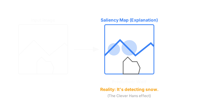
In a famous real-world example, researchers trained a model to classify images of "Husky" dogs versus "Wolf" dogs. The model achieved 90% accuracy. The researchers celebrated. Then, they ran a saliency map.

The map revealed that the model was completely ignoring the animals. It was looking exclusively at the background. In the training data, almost all the wolf pictures were taken in the snow, while the husky pictures were taken on grass. The model hadn't learned to detect wolves; it had learned to detect snow. Without a saliency map, this catastrophic failure would have been deployed to production.

Show Me the Code

Calculating a basic (vanilla) saliency map in PyTorch is surprisingly simple, as it just requires calling .backward() on the input image instead of the loss function.

1import torch2import torch.nn as nn3
4def generate_vanilla_saliency(5    model: nn.Module, 6    image_tensor: torch.Tensor, 7    target_class_idx: int8) -> torch.Tensor:9    """10    Generates a basic gradient saliency map for an image.11    """12    model.eval()13    14    # 1. We need gradients for the input image, not the weights!15    image_tensor.requires_grad_()16    17    # 2. Forward pass18    logits = model(image_tensor)19    20    # 3. Get the score for the specific class we care about21    target_score = logits[0, target_class_idx]22    23    # 4. Backward pass to calculate gradients back to the image24    model.zero_grad()25    target_score.backward()26    27    # 5. The saliency map is the absolute value of the image gradients28    # We take the max across color channels (RGB) to get a 2D heatmap29    saliency_map = image_tensor.grad.abs().squeeze().max(dim=0)[0]30    31    return saliency_map32
33# The resulting 2D tensor is then plotted using matplotlib.imshow(cmap='hot')

Watch Out For

Noisy Gradients

Basic (vanilla) saliency maps generated via direct gradients are often incredibly noisy. They look like television static spread across the image, making it hard to tell what the model is actually focusing on. To get usable, smooth heatmaps, modern computer vision pipelines almost exclusively use advanced variants like grad-cam or integrated-gradients.

The Quick Version

Explainability tools for tabular data are useless for images, because knowing which specific pixel triggered a prediction is not human-readable.
Saliency maps solve this by overlaying a heatmap directly onto the original image.
They are calculated by taking the gradient of the prediction with respect to the input image, mathematically proving which pixels drove the decision.
They are absolutely essential for catching the "Clever Hans" effect—proving that your model actually learned to detect the object, rather than just memorizing background artifacts (like snow or hospital watermarks).