Core ML

Second-Order Optimization

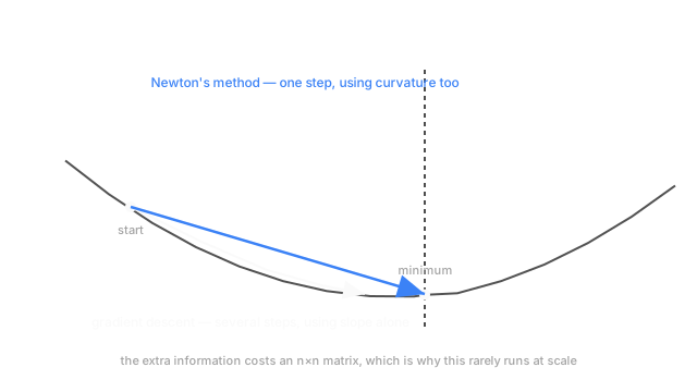
First-order methods only feel the slope underfoot. Second-order methods use curvature too, cutting steps needed sharply, at a memory cost that rules them out at scale.

On a bowl-shaped loss, gradient descent takes several small steps toward the bottom while Newton's method uses the surface's curvature to jump straight there in one step

Why Does This Exist?

Gradient descent only ever asks one question at the current point: which direction is downhill, and how steep is it. That's the gradient — a vector of first derivatives — and it's enough to take a step, but it says nothing about whether the slope is about to flatten out or keep steepening. Two points can have the exact same gradient magnitude and require completely different step sizes to reach the minimum efficiently, because the curvature of the surface around them is different, and the gradient alone can't see that.

Second-order methods use the second derivative — how the slope itself is changing — to answer that missing question directly. On a well-behaved surface, that extra information can cut the number of steps needed from dozens down to one or two. The catch, and it's a large one, is what that information costs to compute and store at the size a modern neural network actually is.

Think of It Like This

Walking downhill blind versus with a map of the terrain

Walking down an unfamiliar hillside in fog, feeling only the slope under your feet at each step, you take a step, feel the new slope, take another — cautious, incremental, and it works, but it takes many small steps to reach the bottom. That's gradient descent: first-order information only, one step at a time.

Now imagine the fog lifts and you can see the whole hillside's shape at once — not just which way is down from here, but how the slope curves ahead, where it's about to level out, where it steepens. With that shape in view, you can often walk in a straight line and land almost exactly at the bottom in far fewer strides. Seeing the shape, not just the slope, is what curvature information buys — and mapping that shape over the whole hillside is expensive.

How It Actually Works

Newton's method

Newton's method updates using both the gradient $\nabla f(\theta)$ and the Hessian matrix $H$ of second partial derivatives:

\theta_{t+1} = \theta_t - H^{-1} \nabla f(\theta_t)

For a purely quadratic function, this converges in exactly one step, because the Hessian fully describes the entire curvature of a quadratic surface and $H^{-1}\nabla f$ points precisely at the minimum. Real loss surfaces aren't quadratic everywhere, but locally, near a minimum, they're often close enough that Newton's method converges in dramatically fewer iterations than gradient descent — when it's computable at all.

The cost that rules it out at scale

The Hessian of a function with $n$ parameters is an $n \times n$ matrix. For a model with 7 billion parameters, that's roughly $4.9 \times 10^{19}$ entries — computing it, let alone inverting it, is not something any hardware built to date can do. This is the entire reason second-order methods stay confined to small models and specific sub-problems rather than displacing first-order methods for training anything at modern scale.

The compromises that make curvature usable anyway

Quasi-Newton methods, most commonly L-BFGS, never build the Hessian at all. They approximate $H^{-1}$ from a short history of recent gradients and parameter changes, updating that approximation incrementally instead of computing curvature exactly. L-BFGS is genuinely used in practice — for small-to-medium models, for fine-tuning specific layers, and inside some classical ML solvers — precisely because it keeps a sliver of second-order benefit at a memory cost closer to a first-order method.

Natural gradient descent takes a different route: instead of the raw parameter-space Hessian, it uses the Fisher information matrix to rescale the gradient step according to how the distribution the model represents changes, not how the raw parameters do. It's a curvature-aware step motivated the same way Newton's method is, without requiring the full Hessian.

Adam's diagonal approximation is the version almost everyone is already using without calling it second-order: Adam's second moment $v_t$ is a coarse, purely diagonal stand-in for curvature information — it captures how much each parameter's own gradient varies, but none of the interaction between parameters that the full Hessian holds. It's a small fraction of what a true second-order method sees, but it's cheap enough to run on every parameter of a large model, which is the trade every method on this page is making in one direction or another.

Show Me the Code

Gradient descent versus Newton's method on the same 1D quadratic, showing the gap in steps needed.

1def grad(x: float, target: float = 3.0) -> float:2    return 2 * (x - target)3
4
5def hessian(x: float) -> float:6    return 2.0  # constant for f(x) = (x - target)^27
8
9x_gd, lr = 10.0, 0.310for _ in range(5):11    x_gd -= lr * grad(x_gd)12
13x_newton = 10.014x_newton -= grad(x_newton) / hessian(x_newton)15
16print(f"gradient descent, 5 steps: x = {x_gd:.4f}")17print(f"Newton's method,  1 step:  x = {x_newton:.4f}")18# -> gradient descent, 5 steps: x = 3.071719# -> Newton's method,  1 step:  x = 3.0000

One Newton step lands exactly on the minimum of this quadratic; five gradient descent steps get close but haven't arrived yet — the curvature information is doing real work here, on a problem simple enough to compute it for.

Watch Out For

Assuming a curvature-aware method always beats a first-order one

Newton's method exactly solves quadratics in one step, but real loss surfaces have saddle points and regions where the Hessian isn't positive definite — and in those regions, a raw Newton step can move toward a saddle rather than away from it. Second-order methods need safeguards (trust regions, damping) to stay reliable off the tidy bowl-shaped case this page's diagram simplifies to.

Reaching for L-BFGS on a model sized for stochastic minibatch training

L-BFGS assumes a consistent, low-noise gradient across calls — it works well with full-batch or low-noise objectives, which is why it shows up in classical ML solvers. Applied naively to noisy minibatch gradients from a large neural network, its curvature approximation gets built from inconsistent information and degrades rather than helps, which is a large part of why Adam remains the default there instead.

The Quick Version

Gradient descent uses only the slope at each point; second-order methods also use curvature, the rate at which the slope itself changes.
Newton's method reaches a quadratic's minimum in one step, using the inverse Hessian to point directly at it.
The full Hessian is an $n \times n$ matrix — computationally out of reach for any model at modern scale.
Quasi-Newton methods like L-BFGS approximate curvature from recent gradient history instead of computing the Hessian exactly.
Adam's second moment is a cheap, diagonal-only stand-in for curvature — the version of this idea already running in most training loops.