Math

Jacobian and Hessian

One matrix holds every first derivative of a function with many inputs and outputs; another holds every second derivative and tells you which way the surface curves.

Frameworks never build the full matrix of derivatives because one layer's would hold sixteen million numbers; they compute a vector multiplied by it instead, which costs one vector in and one vector out

Why Does This Exist?

Two questions that come up constantly and both need this page.

"Why is my training slow when the gradient is clearly not zero?" Because the loss surface is stretched — steep in some directions and nearly flat in others — and a single learning rate cannot suit both. The stretch factor is the Hessian's condition number, and it is the honest explanation for a plateau that is not a minimum.

"What does autodiff actually compute?" Not a gradient, in general. It computes a vector-Jacobian product, and that distinction is why torch.autograd.grad needs a grad_outputs argument for non-scalar outputs, why jacrev and jacfwd exist as separate functions, and why per-sample gradients are awkward.

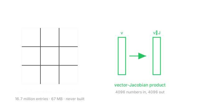
Both objects also explain themselves through size. One layer's Jacobian would hold 16.7 million numbers and a 7-billion-parameter Hessian would hold $4.9 \times 10^{19}$ . Nobody builds either, and understanding what is computed instead is most of the practical content here.

Think of It Like This

A mixing desk, and how sensitive it is

You are at an audio desk with several input faders and several output meters. Move one fader and every meter twitches by a different amount.

The Jacobian is the full table of those sensitivities: one row per meter, one column per fader, each entry saying how much that meter moves per unit of that fader. It completely describes the desk's behaviour for small adjustments — and note it is rectangular, because there is no reason the number of faders equals the number of meters.

Now a different question about a single meter. As you push one fader up, does its response accelerate or level off? And does pushing two faders together do something different from pushing each alone? Those are curvature questions, and the Hessian is the table of answers: one row and column per fader, entry $(i,j)$ describing how fader $i$ and fader $j$ interact.

The Hessian is square and symmetric, because "how does $i$ affect the effect of $j$ " is the same question as the reverse. And it only makes sense for one output at a time, which is why models have a Hessian of their scalar loss and not of their predictions.

How It Actually Works

The Jacobian: all first derivatives

For $f: \mathbb{R}^{n} \to \mathbb{R}^{m}$ , the Jacobian is $m \times n$ with

J_{ij} = \frac{\partial f_i}{\partial x_j}

In plain words: row $i$ describes output $i$ 's sensitivity to every input. Shape is worth stating explicitly — outputs down, inputs across.

A gradient is the special case $m = 1$ : a single row, usually written as a column vector. So the gradient is a Jacobian with one output, which is why training — with its scalar loss — gets a gradient rather than a matrix.

Jacobians compose by multiplication, which is the chain rule for multi-output functions: $J_{g \circ f} = J_g J_f$ . That product is exactly what a backward pass does at every layer.

Why nobody builds one

A layer mapping 4,096 inputs to 4,096 outputs has a Jacobian with $4096^2 = 16{,}777{,}216$ entries — 67 MB in float32, per layer, per example. A hundred layers and a batch of 32 puts you in the hundreds of gigabytes.

So autodiff computes products with the Jacobian instead of the Jacobian itself:

Vector-Jacobian product (VJP), $v^{T}J$ — reverse mode. Costs about one function evaluation, no matrix built. This is .backward().
Jacobian-vector product (JVP), $Jv$ — forward mode. Also one evaluation.

The reason a scalar loss gives you a gradient for free is that $v = [1]$ makes the VJP equal the gradient. For a non-scalar output there is no canonical $v$ , which is why PyTorch demands you supply one. A full Jacobian requires $m$ VJPs or $n$ JVPs — hence jacrev (cheap when outputs are few) and jacfwd (cheap when inputs are few).

The Hessian: all second derivatives

For a scalar function $f: \mathbb{R}^{n} \to \mathbb{R}$ :

H_{ij} = \frac{\partial^2 f}{\partial x_i \partial x_j}

It is $n \times n$ and symmetric for any twice-continuously-differentiable function, because the order of partial differentiation does not matter. Symmetry means it has real eigenvalues and orthogonal eigenvectors, so everything from eigenvalues applies.

Equivalently, the Hessian is the Jacobian of the gradient.

What the Hessian tells you

It classifies stationary points. Where the gradient is zero, the Hessian's definiteness decides: positive definite is a minimum, negative definite a maximum, indefinite a saddle. In high dimensions minima are rare, because every one of $n$ eigenvalues must be positive.

It explains slow training. The condition number $\kappa = \lambda_{\max}/\lambda_{\min}$ measures how stretched the surface is. Gradient descent's convergence rate degrades directly with $\kappa$ : a large one means zigzagging across a narrow valley rather than travelling along it. This, not the gradient magnitude, is why training plateaus.

It sets the ideal step. Along an eigenvector with eigenvalue $\lambda$ , the largest stable gradient-descent learning rate is $2/\lambda$ . So the largest eigenvalue caps your global learning rate while the smallest determines how slowly the flattest direction progresses — and a large $\kappa$ means no single rate serves both. That gap is what adaptive optimisers exist to close.

Worked example

A Jacobian. Take $f(x, y) = [x^2 y,\; x + y^2]$ , so $n = 2$ and $m = 2$ .

Differentiate each output with respect to each input:

J = \begin{bmatrix} 2xy & x^2 \\ 1 & 2y \end{bmatrix}

At $(x, y) = (2, 3)$ : $2xy = 12$ , $x^2 = 4$ , and $2y = 6$ , giving

J(2,3) = \begin{bmatrix} 12 & 4 \\ 1 & 6 \end{bmatrix}

Note it is not symmetric — Jacobians generally are not. Its determinant is $72 - 4 = 68$ , the local volume scaling factor.

A Hessian. Take the scalar $g(x, y) = x^2 + 3y^2 + xy$ .

First derivatives: $\partial g/\partial x = 2x + y$ and $\partial g/\partial y = 6y + x$ . Differentiate again:

H = \begin{bmatrix} 2 & 1 \\ 1 & 6 \end{bmatrix}

Symmetric, as promised, and constant here because $g$ is quadratic. The eigenvalues solve $(2-\lambda)(6-\lambda) - 1 = 0$ , so $\lambda^2 - 8\lambda + 11 = 0$ and:

\lambda = \frac{8 \pm \sqrt{64 - 44}}{2} = 4 \pm \sqrt{5} \approx 6.236,\; 1.764

Check both identities: trace is $2 + 6 = 8$ and $6.236 + 1.764 = 8$ ✓; determinant is $12 - 1 = 11$ and $6.236 \times 1.764 = 11.0$ ✓.

Both eigenvalues are positive, so $H$ is positive definite, so $g$ is convex with a single minimum. The condition number is $6.236/1.764 \approx 3.54$ — mild, and this surface would optimise easily. Real loss surfaces reach $\kappa$ in the thousands, which is the whole difficulty.

The maximum stable learning rate here is $2/\lambda_{\max} = 2/6.236 \approx 0.32$ . Above that, gradient descent diverges along the steepest eigenvector.

Show Me the Code

1import numpy as np2
3
4def jacobian_f(x: float, y: float) -> np.ndarray:5    # f(x,y) = [x^2 y, x + y^2] -> shape (outputs=2, inputs=2)6    return np.array([[2 * x * y, x**2], [1.0, 2 * y]])7
8
9H = np.array([[2.0, 1.0], [1.0, 6.0]])       # Hessian of x^2 + 3y^2 + xy10
11print(jacobian_f(2, 3).tolist())              # -> [[12.0, 4.0], [1.0, 6.0]]12print(round(float(np.linalg.det(jacobian_f(2, 3))), 6))   # -> 68.013
14vals = np.linalg.eigvalsh(H)                  # eigh: symmetric, real, ascending15print(np.round(vals, 4))                       # -> [1.7639 6.2361]  = 4 -/+ sqrt(5)16print(round(float(vals.sum()), 6), round(float(np.trace(H)), 6))       # -> 8.0 8.017print(round(float(np.prod(vals)), 6), round(float(np.linalg.det(H)), 6))  # -> 11.0 11.018print(round(float(vals[-1] / vals[0]), 4))     # -> 3.5352  condition number19print(round(2 / float(vals[-1]), 4))           # -> 0.3208  max stable learning rate20
21# The size argument for never materialising a Jacobian.22n = 409623print(n * n, round(n * n * 4 / 1024**2, 1))    # -> 16777216 64.0  (MB, float32)

Every number matches the hand calculation, including the eigenvalues as $4 \pm \sqrt{5}$ and the trace and determinant checks.

Watch Out For

Asking for a full Jacobian when you wanted a vector product

torch.autograd.functional.jacobian and jax.jacrev build the whole matrix, and the cost scales with the number of outputs — one reverse pass each. Call it on a layer with thousands of outputs and you have queued thousands of backward passes and allocated a matrix in the tens of megabytes.

The usual symptom is code that works on a toy example and becomes unusably slow or exhausts memory at real width. And it is almost always avoidable, because the downstream computation only needs a product with the Jacobian, not the Jacobian.

Recognise the pattern. If your next step is J @ v or v @ J, use a JVP or VJP directly — torch.func.jvp, torch.func.vjp, jax.jvp, jax.vjp — and pay one pass instead of $n$ or $m$ . Gradient penalties, Hessian-vector products, influence functions and Fisher-vector products are all products in disguise.

Pick the right direction, too: jacrev costs one pass per output, jacfwd one per input. For a function with 3 inputs and 4,096 outputs, forward mode is a thousand times cheaper. Getting this backwards is a common and invisible performance bug.

Computing a Hessian when a Hessian-vector product would do

The Hessian is $n \times n$ , so it is out of reach the moment $n$ is a real parameter count — and yet almost every algorithm that appears to need one actually needs $Hv$ for some vector $v$ .

The Pearlmutter trick computes $Hv$ at roughly the cost of two gradient evaluations, with no matrix formed. The insight is that $Hv$ is the directional derivative of the gradient along $v$ , so you differentiate the scalar $\nabla\mathcal{L}^{T}v$ once more. In PyTorch that is a grad call on the dot product of the gradient with $v$ , using create_graph=True on the first pass.

That single primitive covers most of the field. Conjugate-gradient Newton methods need only $Hv$ . Estimating the largest eigenvalue by power iteration needs only $Hv$ . Trust-region methods, influence functions, and curvature-based pruning criteria are all built on it.

Two related warnings. Do not estimate curvature by finite-differencing gradients unless you have to — it inherits catastrophic cancellation and needs a carefully chosen step. And check what your library means by "Hessian": K-FAC, Adam's second moment, and the Gauss-Newton approximation are all different approximations with different failure modes, and treating them as interchangeable produces results that are hard to explain.

The Quick Version

Jacobian: all first derivatives of a multi-output function, shape $m \times n$ , outputs down and inputs across.
A gradient is a Jacobian with one output. Jacobians compose by multiplication — that is the chain rule.
Never build one: a 4096→4096 layer's Jacobian is 16.7M entries, 67 MB per example.
Autodiff computes VJP ( $v^{T}J$ , reverse mode) or JVP ( $Jv$ , forward mode) at about one function evaluation.
A scalar loss makes $v = [1]$ , so the VJP is the gradient. Non-scalar outputs need you to supply $v$ .
jacrev costs one pass per output; jacfwd one per input. Choose by which is smaller.
Hessian: all second derivatives of a scalar function, $n \times n$ and always symmetric. It is the Jacobian of the gradient.
Its definiteness classifies a stationary point; in high dimensions saddles dominate because every eigenvalue must be positive for a minimum.
The condition number $\lambda_{\max}/\lambda_{\min}$ explains slow training better than gradient magnitude does.
Max stable learning rate along an eigendirection is $2/\lambda$ , so $\lambda_{\max}$ caps your global rate.
Use Hessian-vector products via the Pearlmutter trick — about two gradient evaluations, no matrix.