Math

Constrained Optimisation and Duality

Optimising with a rule you cannot break — and the discovery that the multiplier enforcing the rule is also the price of relaxing it.

The best point on a constraint is where a contour of the objective just touches it: push to a better contour and you leave the constraint, so at the optimum the two gradients point the same way

Why Does This Exist?

Support vector machines are usually taught as "maximise the margin", and then the derivation abruptly switches to a completely different problem — one over per-example coefficients, where most of them turn out to be zero and the data appears only inside dot products. That switch is not a trick or a convenience. It is Lagrangian duality, and without this page it has to be accepted on faith.

Three things it explains:

Why SVMs have "support vectors" at all. The KKT conditions force most multipliers to zero, so only the examples on the boundary matter. That is a consequence of the mathematics, not a design choice.
Why the kernel trick is possible. In the dual problem the data appears only as dot products, so you can replace them with a kernel and never touch the feature space.
What a multiplier means. It is a shadow price — the rate at which loosening a constraint improves your objective. That reading makes constrained problems interpretable rather than mechanical.

More broadly: regularisation, fairness constraints, KL-constrained policy updates in RLHF, and trust-region methods are all constrained optimisation, and the multiplier is the knob.

Think of It Like This

Buying the biggest rectangle you can afford in fence

You want to enclose the largest possible area, and you have exactly 100 metres of fence. More area is always better; the fence is fixed.

Start with any rectangle and try to improve it. Make it wider and you must make it shorter to stay within the fence. Sometimes that trade gains area, sometimes it loses. You are at the best rectangle when no trade helps — when the gain from widening exactly cancels the loss from shortening.

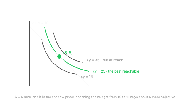
Geometrically, that is tangency. Picture curves of constant area on a plot of width against height. You want the highest one you can reach, and the constraint is a straight line. The best you can do is the curve that just touches the line — any better curve misses it entirely. At that touching point the two curves share a tangent, so their gradients are parallel, and the multiplier is the ratio between them.

Now the part worth keeping. Ask what one extra metre of fence is worth. You can compute it, and the answer is exactly the multiplier. It was never just bookkeeping — it was the price all along.

How It Actually Works

To minimise $f(x)$ subject to $g(x) = 0$ , build the Lagrangian:

\mathcal{L}(x, \lambda) = f(x) - \lambda\, g(x)

Then set all its partial derivatives — with respect to $x$ and $\lambda$ — to zero. Differentiating by $\lambda$ recovers the constraint; differentiating by $x$ gives the stationarity condition:

\nabla f = \lambda \nabla g

In plain words: at the optimum, the objective's gradient is parallel to the constraint's gradient. If it were not, some component of $\nabla f$ would lie along the constraint surface, and you could slide along the constraint and improve — so you would not be at the optimum. That argument is the method.

The trick is that a constrained problem in $n$ variables has become an unconstrained problem in $n + 1$ .

Inequalities need the KKT conditions

Real problems have inequalities, $g(x) \le 0$ , and those add two requirements. For minimising $f$ subject to $g_i(x) \le 0$ :

Stationarity — $\nabla f + \sum_i \lambda_i \nabla g_i = 0$ .
Primal feasibility — $g_i(x) \le 0$ .
Dual feasibility — $\lambda_i \ge 0$ .
Complementary slackness — $\lambda_i\, g_i(x) = 0$ for every $i$ .

The fourth is the one that does the work. It says that for each constraint, either the multiplier is zero or the constraint is tight. A constraint you are not pressing against has no influence, so its price is zero; a constraint that binds has a positive price.

That single condition produces support vectors. In an SVM, examples comfortably inside their margin have inactive constraints, so their multipliers are zero and they drop out of the solution entirely. Only the examples on the margin have nonzero multipliers — and those are the support vectors. Sparsity was forced by the mathematics.

The dual problem

Minimising the Lagrangian over $x$ for a fixed $\lambda$ gives the dual function, and maximising that over $\lambda \ge 0$ is the dual problem. It always provides a lower bound on the primal minimum — weak duality — and for convex problems satisfying mild conditions the bound is tight, which is strong duality.

Why bother? Three reasons, all practical:

The dual can be easier. The SVM dual is a quadratic program in $n$ variables with simple box constraints, which is far more tractable than the primal in high-dimensional feature space.
The dual can reveal structure. The SVM dual contains the data only as $x_i^{T}x_j$ . Replace that dot product with a kernel and you operate in an implicit high-dimensional space at no cost. The kernel trick is a consequence of duality, not an independent idea.
The gap is a certificate. The difference between primal and dual values bounds how far from optimal you are, which is how interior-point solvers know when to stop.

The multiplier is a price

The most useful interpretation. If the constraint is $g(x) = c$ , then:

\frac{\partial f^{*}}{\partial c} = \lambda

In plain words: the multiplier is the rate at which the optimal value improves as you relax the constraint by one unit. Economists call it the shadow price, and it makes the number interpretable — "this constraint is costing me 5 units of objective per unit of tightness".

This is also why regularisation strength and a constraint budget are two views of one thing. Minimising $f(x) + \lambda \lVert x \rVert^2$ is the Lagrangian of minimising $f(x)$ subject to $\lVert x \rVert^2 \le c$ , and every $\lambda$ corresponds to some $c$ . Weight decay is a constrained problem in disguise, which is the same duality that makes KL-constrained policy optimisation in RLHF equivalent to a KL penalty.

Worked example

Maximise $f(x,y) = xy$ subject to $x + y = 10$ .

Form the Lagrangian:

\mathcal{L} = xy - \lambda(x + y - 10)

Set the partial derivatives to zero:

\frac{\partial \mathcal{L}}{\partial x} = y - \lambda = 0, \qquad \frac{\partial \mathcal{L}}{\partial y} = x - \lambda = 0

So $x = \lambda$ and $y = \lambda$ . Substituting into the constraint gives $2\lambda = 10$ , hence $\lambda = 5$ and $x = y = 5$ , with $f = 25$ .

Sanity-check by trying other splits: $4 \times 6 = 24$ and $3 \times 7 = 21$ , both worse than 25 ✓. Equal shares win, which is what the tangency in the diagram shows.

Now the shadow price, which is the point. Loosen the constraint to $x + y = 11$ . By the same algebra $x = y = 5.5$ and $f = 30.25$ — an increase of $5.25$ for one extra unit of budget, and $\lambda = 5$ predicted 5.

The prediction is first-order, and you can confirm it exactly. With a general budget $c$ , the optimum is $x = y = c/2$ so $f^{*} = c^2/4$ , and:

\frac{df^{*}}{dc} = \frac{c}{2} = 5 \quad \text{at } c = 10

Exactly $\lambda$ . The multiplier was never bookkeeping.

Show Me the Code

1import numpy as np2from scipy.optimize import minimize3
4# Maximise xy subject to x + y = 10, i.e. minimise -xy.5res = minimize(6    fun=lambda v: -v[0] * v[1],7    x0=np.array([1.0, 9.0]),8    constraints=[{"type": "eq", "fun": lambda v: v[0] + v[1] - 10}],9)10print(np.round(res.x, 6).tolist(), round(-res.fun, 6))   # -> [5.0, 5.0] 25.011
12# The optimum for a general budget c is c^2/4, so df*/dc = c/2 = lambda.13f_star = lambda c: c**2 / 414print(f_star(10), f_star(11), round(f_star(11) - f_star(10), 4))  # -> 25.0 30.25 5.2515print(round((f_star(10.001) - f_star(9.999)) / 0.002, 6))          # -> 5.0  == lambda16
17# Complementary slackness: an inactive constraint has a zero multiplier.18# Minimise x^2 subject to x >= -1. The bound is slack, so lambda = 0 and x = 0.19res2 = minimize(lambda v: v[0] ** 2, x0=np.array([0.5]),20                constraints=[{"type": "ineq", "fun": lambda v: v[0] + 1}])21print(round(float(res2.x[0]), 6))                         # -> 0.0  bound never binds

The solver lands on $(5,5)$ with $f = 25$ , and the numerical derivative of the optimum with respect to the budget returns exactly 5 — the multiplier, confirmed as a shadow price.

Watch Out For

Treating a stationary point of the Lagrangian as a solution

Setting $\nabla\mathcal{L} = 0$ finds candidates, not answers. The Lagrangian's stationary points include constrained minima, constrained maxima, and saddles, and the equations do not distinguish them.

In the worked example the algebra gave $x = y = 5$ and nothing in it said "maximum". It happened to be one because $xy$ on that line is concave, which we knew separately. Change the objective and the same procedure can hand you the worst point on the constraint.

There is a second, subtler failure. Lagrange's method requires the constraint gradients to be linearly independent at the solution — a regularity condition. Where it fails, at a cusp or where constraints are redundant, no valid multiplier exists and the method finds nothing, even though a solution does exist.

Three defences. Check second-order conditions on the bordered Hessian, or verify convexity of the problem, which makes any stationary point a global solution. Evaluate all candidates and compare, including the boundary, since with several constraints there are several combinations of active sets. And for anything real, use a solver — scipy.optimize.minimize with constraints, or cvxpy for convex problems, both of which check the conditions properly. Deriving multipliers by hand is for understanding; solvers are for answers.

Assuming the dual solves the primal

Weak duality always holds — the dual optimum is a lower bound on the primal minimum. Strong duality, where they are equal, requires convexity plus a regularity condition such as Slater's, and neither is automatic.

For non-convex problems there is generally a duality gap, and solving the dual gives you a bound rather than a solution. Recover a primal point from a dual solution of a non-convex problem and it may be infeasible or simply not optimal. This matters because neural network training is non-convex, so intuitions imported from SVM duality do not transfer.

The gap is not always bad news. A dual bound tells you how far from optimal you might be, which is genuinely useful — it is how branch-and-bound prunes. But it is a bound, and reporting it as the answer is wrong.

Where this shows up in ML: KL-constrained policy optimisation is usually solved as a penalty because the constrained form is harder, and the two are only equivalent under convexity, so the penalty coefficient must be tuned rather than derived. Similarly, adding a fairness constraint as a penalty term is not the same problem as enforcing it, and a model can satisfy the penalty on average while violating the constraint on subgroups.

The habit: state whether your problem is convex before relying on duality. If it is, the dual is a legitimate route to the answer. If it is not, the dual gives you a bound and a diagnostic.

The Quick Version

Build $\mathcal{L} = f - \lambda g$ and set every partial derivative to zero. A constrained problem in $n$ variables becomes unconstrained in $n+1$ .
Stationarity says $\nabla f = \lambda \nabla g$ : the gradients are parallel at the optimum, which is tangency.
Inequalities need the four KKT conditions: stationarity, primal feasibility, dual feasibility, complementary slackness.
Complementary slackness — either the multiplier is zero or the constraint is tight — is what produces support vectors.
The dual is always a lower bound (weak duality); equality needs convexity plus regularity (strong duality).
The SVM dual contains the data only as dot products, and that is why the kernel trick works.
The multiplier is a shadow price: $\partial f^{*} / \partial c = \lambda$ , the value of one more unit of budget.
Weight decay and a norm constraint are the same problem — every $\lambda$ corresponds to some budget $c$ .
Verified: maximising $xy$ under $x+y=10$ gives $x=y=5$ , $f=25$ , $\lambda=5$ , and relaxing to 11 gains 5.25.
$\nabla\mathcal{L} = 0$ finds candidates, not solutions. Check second-order conditions or convexity.
Non-convex problems have a duality gap, so a dual solution is a bound rather than an answer.