Math

Linear Transformations

A matrix is not a grid of numbers, it is an instruction for reshaping space — and reading its columns tells you exactly where the axes end up.

A matrix is a recipe for reshaping space: it sends the unit square to a parallelogram, and its determinant is exactly the factor by which area changes

Why Does This Exist?

A dense layer is a linear transformation. So is an embedding lookup, every projection inside attention, and every convolution. If you understand what a matrix does to space rather than just how to multiply one, a large amount of deep learning stops being arbitrary.

Three things this page buys you concretely.

Why depth needs nonlinearity. Stacking linear transformations gives you another linear transformation — the composition of two matrices is just their product. So a hundred-layer network without activation functions has exactly the capacity of a single layer. That is not a heuristic; it is a one-line consequence of composition.

What the determinant means. It is the factor by which volume changes, and a determinant of zero means the transformation flattened space and destroyed information. This is the quantity normalising flows track as $\log|\det J|$ , and knowing what it is makes those models legible.

Why "linear layer" is a misnomer. A layer with a bias is affine, not linear, and the distinction has real consequences for what you can fold, invert, and compose.

Think of It Like This

A photocopier with skew and zoom dials

Picture a photocopier that can do more than shrink and enlarge. It has dials for horizontal stretch, vertical stretch, rotation, and skew. Feed in a square and it hands back a parallelogram.

Two properties define what this machine is allowed to do. Straight lines stay straight — nothing gets curved. And the origin stays put — the copy is never shifted bodily across the page. Any machine obeying those two rules is a linear transformation, and every such machine is describable by a matrix.

Now the useful part. To work out what the machine does, you do not need to test every possible input. Feed in just the two unit arrows, one along each axis, and see where they land. Those two answers are the columns of the matrix, and everything else follows because any shape is built from combinations of them.

And the area of the output parallelogram, divided by the area of the square you put in, is the determinant. Set a dial such that the parallelogram collapses to a line and the determinant is zero — you have lost a dimension, and no setting of the dials can undo it.

How It Actually Works

A map $T$ is linear when it respects addition and scaling:

T(u + v) = T(u) + T(v), \qquad T(cv) = c\,T(v)

In plain words: transforming a sum gives the sum of the transforms, and scaling before is the same as scaling after. Setting $c = 0$ in the second rule forces $T(0) = 0$ — a linear map must fix the origin, which is the rule bias terms break.

Every linear map from $\mathbb{R}^n$ to $\mathbb{R}^m$ is a matrix, and the columns of that matrix are where the basis vectors go. For $A = \begin{bmatrix} 2 & 1 \\ 0 & 1 \end{bmatrix}$ , the first column $[2,0]$ is where $[1,0]$ lands and the second column $[1,1]$ is where $[0,1]$ lands. Reading a matrix column-wise tells you what it does, which is the single most useful habit on this page.

Composition is multiplication

Apply $A$ then $B$ and the result is the single transformation $BA$ :

B(Ax) = (BA)x

In plain words: chaining transformations is multiplying their matrices, right to left. This is where non-commutativity gets its meaning — rotating then stretching is genuinely a different operation from stretching then rotating, and $AB \neq BA$ is that fact in algebra.

It is also the proof that depth without nonlinearity is pointless. A stack of $k$ dense layers computes $W_k \cdots W_2 W_1 x$ , which is one matrix. Every activation function exists to break this collapse.

The determinant is a volume factor

For a square matrix, $\det A$ is the signed factor by which volume changes. In 2D it is the area of the parallelogram the unit square becomes; in 3D the volume of the parallelepiped the unit cube becomes.

The sign carries orientation: negative means space was flipped, like a reflection. And three consequences matter:

$\det A = 0$ means volume collapsed to nothing — the transformation squashed space into a lower dimension. Information is destroyed, and no inverse exists. This is rank deficiency seen geometrically.
$\det(AB) = \det A \cdot \det B$ , because volume factors multiply along a chain.
$|\det A| > 1$ expands, $< 1$ contracts. Repeated application therefore blows up or vanishes, which is one way to see why the product of many layers is unstable.

For a $2 \times 2$ matrix, $\det \begin{bmatrix} a & b \\ c & d \end{bmatrix} = ad - bc$ .

Affine is not linear, and your layers are affine

A dense layer computes $Wx + b$ . The $Wx$ part is linear; adding $b$ shifts the origin, which breaks $T(0) = 0$ . The combination is an affine transformation.

The distinction is not pedantry:

Composition still works — affine composed with affine is affine, which is why the depth-collapse argument survives bias terms.
Folding requires care. Merging BatchNorm into a preceding convolution at inference time works precisely because both are affine, but you have to carry the bias through correctly; dropping it is a real and silent bug.
The standard trick is homogeneous coordinates: append a 1 to the input and put $b$ in an extra column of $W$ . Now the affine map is a single linear map in one higher dimension, which is how graphics libraries handle translation.

Worked example

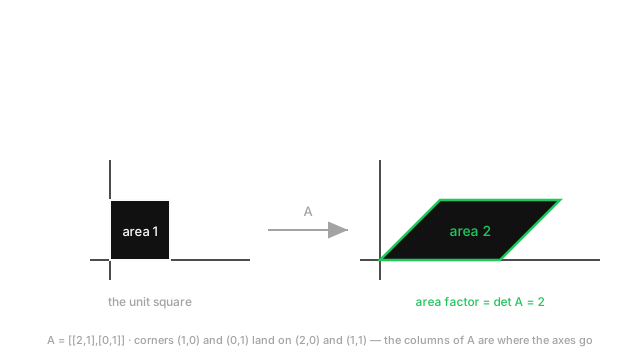
Take $A = \begin{bmatrix} 2 & 1 \\ 0 & 1 \end{bmatrix}$ and follow the unit square's corners.

Read the columns first: $[1,0]$ goes to $[2,0]$ and $[0,1]$ goes to $[1,1]$ . So the transformation stretches horizontally and skews the vertical axis to the right.

The four corners:

$[0,0] \mapsto [0,0]$ — the origin is fixed, as linearity requires.
$[1,0] \mapsto [2 \cdot 1 + 1 \cdot 0,\; 0 \cdot 1 + 1 \cdot 0] = [2, 0]$
$[1,1] \mapsto [2 + 1,\; 0 + 1] = [3, 1]$
$[0,1] \mapsto [0 + 1,\; 0 + 1] = [1, 1]$

That is the parallelogram in the diagram. Its determinant:

\det A = 2 \times 1 - 1 \times 0 = 2

In plain words: every region doubles in area. Check it independently — the parallelogram has base 2 (from $[0,0]$ to $[2,0]$ ) and vertical height 1, so its area is $2 \times 1 = 2$ , against the unit square's 1. Ratio 2, matching the determinant.

Now compose $A$ with itself. $A^2 = \begin{bmatrix} 4 & 3 \\ 0 & 1 \end{bmatrix}$ , and $\det A^2 = 4 = 2^2$ , exactly as the multiplicative rule predicts.

Contrast with $S = \begin{bmatrix} 1 & 2 \\ 2 & 4 \end{bmatrix}$ : $\det S = 4 - 4 = 0$ . This one flattens the plane onto a line, and its output has no area at all.

Show Me the Code

1import numpy as np2
3A = np.array([[2.0, 1.0], [0.0, 1.0]])4square = np.array([[0, 1, 1, 0], [0, 0, 1, 1]], dtype=float)  # (2, 4) corners5
6print((A @ square).T.tolist())     # -> [[0,0], [2,0], [3,1], [1,1]]7print(A[:, 0], A[:, 1])            # -> [2. 0.] [1. 1.]  where each axis lands8print(round(np.linalg.det(A), 10))                 # -> 2.0   area factor9print(round(np.linalg.det(A @ A), 10))             # -> 4.0   = 2 * 210
11# Depth without nonlinearity collapses to ONE matrix.12W1, W2, W3 = (np.random.default_rng(k).standard_normal((3, 3)) for k in (1, 2, 3))13x = np.array([1.0, 2.0, 3.0])14print(np.allclose(W3 @ (W2 @ (W1 @ x)), (W3 @ W2 @ W1) @ x))   # -> True15
16print(round(np.linalg.det(np.array([[1.0, 2.0], [2.0, 4.0]])), 10))  # -> 0.0

The corner coordinates and the determinant of 2 match the hand calculation. The allclose line is the depth-collapse argument as an executable check.

Watch Out For

Treating a dense layer as a linear map when reasoning about composition

nn.Linear computes $Wx + b$ , which is affine. Most of the time this does not bite, and then occasionally it does — hard.

The clearest case is merging layers for inference. Folding BatchNorm into a convolution is standard and safe, but the fold has two parts: the scale multiplies into the weights, and the shift combines into the bias. Implement only the weight half and the model still runs, still produces sensible-looking outputs, and is quietly wrong — typically a few percent of accuracy, which is easy to attribute to something else.

The second case is inversion. People reason "the layer is a matrix, so invert the matrix", and forget to subtract the bias first. The inverse of $x \mapsto Wx + b$ is $y \mapsto W^{-1}(y - b)$ , and dropping the subtraction gives an offset error that grows with the bias magnitude.

The habit that avoids both: write out the affine form explicitly whenever you compose, fold, or invert. If a derivation on a whiteboard says $W_2 W_1 x$ , check whether the biases were dropped on purpose or by accident.

Computing a determinant directly on a large matrix

The determinant multiplies $n$ numbers of similar magnitude, so it overflows and underflows catastrophically at very modest sizes.

Take a $1000 \times 1000$ matrix whose singular values average 2. Its determinant is around $2^{1000} \approx 10^{301}$ , right at the edge of float64, and average 10 puts it at $10^{1000}$ — plain inf. In the other direction, average 0.5 gives $10^{-301}$ , which underflows to exactly 0 and then reads as "singular" when the matrix is perfectly well conditioned.

So np.linalg.det returning 0.0 or inf on a large matrix tells you almost nothing about the matrix. Two correct tools instead. np.linalg.slogdet returns the sign and the log of the absolute determinant, which stays in range — and it is what any log-likelihood involving a determinant should use, including the $\log|\det J|$ term in a normalising flow. And for the question "is this invertible", use np.linalg.matrix_rank or the condition number, both of which work from singular values and do not multiply anything.

The Quick Version

Linear means additivity and scaling are preserved, which forces $T(0) = 0$ .
Every linear map is a matrix, and its columns are where the basis vectors land. Read matrices column-wise.
Composing transformations is multiplying matrices, right to left. Non-commutativity is why order matters physically.
A stack of dense layers without activations collapses to one matrix. That is why nonlinearity exists.
The determinant is the signed volume factor. $\det(AB) = \det A \det B$ .
$\det A = 0$ means space was flattened, information destroyed, no inverse. Same fact as rank deficiency.
A dense layer with bias is affine, not linear. This matters for folding, inverting, and composing.
Homogeneous coordinates turn an affine map into a linear one in one more dimension.
Never compute a determinant directly on a large matrix. Use slogdet, or rank and condition number.