Math

Vector Spaces and Rank

How many genuinely different directions a set of numbers actually contains — usually far fewer than its size suggests, which is the redundancy every compression trick exploits.

Rank counts genuinely new directions, not rows: two vectors lying on the same line span only that line no matter how many you add, which is the redundancy low-rank methods exploit

Why Does This Exist?

Fine-tuning a 7-billion-parameter model on a single consumer GPU should be impossible. The weights alone need more memory than the card has, and the gradients and optimiser state multiply that several times over. LoRA does it anyway, and the reason is this page.

The observation is that a fine-tuning update to a weight matrix does not need all the directions the matrix has room for. Take one $4096 \times 4096$ layer: a full update is 16.7 million numbers. Restrict the update to rank 8 and you store two thin matrices instead, $4096 \times 8$ and $8 \times 4096$ , which is 65,536 numbers — a 256-fold reduction. It works because the useful part of the update genuinely lives in a handful of directions, and rank is the tool that says how many.

The same idea keeps reappearing. PCA keeps the top few directions of your data. Embedding tables are low-rank factorised. Model compression is low-rank approximation. And in the other direction, rank explains failure: when features are linearly dependent, the closed-form regression solution stops existing, and rank is what diagnoses it.

Think of It Like This

Directions in a city, from a lot of instructions

Someone gives you five sets of walking directions from the town square: "three blocks east", "six blocks east", "one block east", "two blocks north", "four blocks north".

Five instructions. But how many places can you actually get to? Only two of them are doing anything new — one east instruction and one north instruction. The others are just the same directions at different lengths, and combining east and north reaches anywhere in the city. So five instructions carry two directions' worth of information.

That count is the rank. The set of everywhere you can reach is the span. And notice you cannot get off the street grid — no combination of east and north gives you altitude, so the whole grid is two-dimensional however many instructions you are handed.

The last piece: if every instruction had been an east one, the rank would be 1 and you could only ever move along a single line. Redundancy is not a curiosity here, it is the thing being measured.

How It Actually Works

A vector space is a set of vectors closed under addition and scaling — add any two members and you stay inside, scale any member and you stay inside. $\mathbb{R}^n$ is the one you use. A subspace is a vector space sitting inside a larger one, and it must contain the origin, because scaling any member by zero has to land somewhere legal.

Three definitions stack on that:

Span — everything reachable by linear combination of a set of vectors. The span of $\{[1,0], [0,1]\}$ is the whole plane; the span of $\{[1,0], [2,0]\}$ is one line.
Linear independence — no vector in the set is a combination of the others. Equivalently, the only way to combine them into the zero vector is with all-zero coefficients.
Basis — an independent set that spans the space. Its size is the dimension, and every basis of the same space has the same size.

Rank

The rank of a matrix is the number of linearly independent rows — which is always identical to the number of linearly independent columns, a genuinely surprising fact. So:

\text{rank}(A) \le \min(m, n)

In plain words: rank cannot exceed either dimension of the matrix. A matrix achieving that bound is full rank; below it, rank-deficient or singular.

The gap between a matrix's size and its rank is exactly the redundancy available to exploit. A $1000 \times 1000$ matrix whose every row is a multiple of the first is rank 1: a million numbers carrying one direction's worth of information.

Null space and the rank–nullity theorem

The null space is every vector the matrix sends to zero:

\mathcal{N}(A) = \{x : Ax = 0\}

In plain words: the directions the matrix destroys. It is always a subspace, and it always contains the zero vector.

The rank–nullity theorem ties the two together. For $A$ with $n$ columns:

\text{rank}(A) + \dim \mathcal{N}(A) = n

In plain words: every input direction is either preserved or destroyed, and the counts add up to the number you started with. A full-rank square matrix has a null space containing only zero — nothing is destroyed, so the map is reversible and $A^{-1}$ exists. A nonzero null space means information is lost and no inverse can exist, because you cannot recover which of many inputs produced the same output.

Why low rank is a saving

A rank- $r$ matrix of shape $m \times n$ factors into an $m \times r$ times an $r \times n$ :

A = BC, \qquad B \in \mathbb{R}^{m \times r},\; C \in \mathbb{R}^{r \times n}

Storage drops from $mn$ to $r(m + n)$ , which is a large win whenever $r \ll \min(m,n)$ . For $m = n = 4096$ and $r = 8$ : from 16,777,216 to 65,536 numbers.

Finding the best rank- $r$ approximation of a matrix that is not exactly low rank is what singular value decomposition does, and it comes with a guarantee that no better rank- $r$ approximation exists.

Worked example

Take two $2 \times 2$ matrices.

A = \begin{bmatrix} 1 & 2 \\ 2 & 4 \end{bmatrix}, \qquad B = \begin{bmatrix} 1 & 2 \\ 3 & 4 \end{bmatrix}

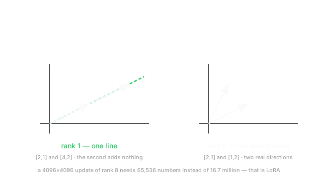
For $A$ , the second row is exactly twice the first. So the rows are dependent, and $\text{rank}(A) = 1$ . Its determinant confirms it: $1 \times 4 - 2 \times 2 = 0$ , and a zero determinant means singular.

Its null space: solve $x + 2y = 0$ , giving $x = -2y$ . Every solution is a multiple of $[-2, 1]$ , so the null space is one-dimensional. Check the theorem: $\text{rank} + \text{nullity} = 1 + 1 = 2 = n$ . Verify by hand that $A$ really does kill that direction — $A[-2, 1]^{T} = [-2 + 2,\; -4 + 4]^{T} = [0, 0]^{T}$ . It does.

For $B$ , the second row is not a multiple of the first. $\det B = 1 \times 4 - 2 \times 3 = -2 \neq 0$ , so $\text{rank}(B) = 2$ , full rank, null space is just the origin, and $B^{-1}$ exists.

The diagram shows the same contrast geometrically: $[2,1]$ and $[4,2]$ lie on one line and span it, while $[2,1]$ and $[1,2]$ span the whole plane.

Show Me the Code

1import numpy as np2
3A = np.array([[1.0, 2.0], [2.0, 4.0]])   # row 2 = 2 x row 14B = np.array([[1.0, 2.0], [3.0, 4.0]])5
6print(np.linalg.matrix_rank(A), np.linalg.matrix_rank(B))   # -> 1 27print(round(np.linalg.det(A), 10), round(np.linalg.det(B), 10))  # -> 0.0 -2.08print(A @ np.array([-2.0, 1.0]))          # -> [0. 0.]  the null-space direction9
10# Rank is a THRESHOLD on singular values, not an exact algebraic test.11noisy = A + 1e-12 * np.random.default_rng(0).standard_normal((2, 2))12print(np.linalg.svd(noisy, compute_uv=False))   # -> [5.0, ~1e-12] not [5.0, 0]13print(np.linalg.matrix_rank(noisy))             # -> 1, because it uses a tolerance14
15# The low-rank saving, in numbers.16m = n = 4096; r = 817print(m * n, r * (m + n), (m * n) // (r * (m + n)))  # -> 16777216 65536 256

The 256× figure is the LoRA saving. The middle block is the pitfall below: with a floating-point perturbation the second singular value is tiny rather than zero, and only a tolerance recovers the right answer.

Watch Out For

Testing for rank deficiency with an exact comparison

Mathematically, rank deficiency means a singular value is exactly zero. In floating point it almost never is.

Read a rank-1 matrix from a CSV, or produce one through any arithmetic, and rounding leaves its smallest singular value at something like $10^{-16}$ rather than 0. So det(A) == 0 is essentially always False, and any code branching on it takes the wrong path on data that is rank-deficient in every way that matters.

np.linalg.matrix_rank gets this right by counting singular values above a tolerance scaled to the matrix size and its largest singular value. Use it rather than a determinant test — determinants also overflow badly for large matrices, since they multiply $n$ numbers together.

The deeper point is that rank is not binary in practice, it is a spectrum. The useful question is rarely "is this singular" but "how many singular values are large enough to matter", which is a modelling decision about your tolerance. That reframing is what makes low-rank approximation work at all: real matrices are full rank with a rapidly decaying spectrum, not exactly low rank.

Feeding linearly dependent features to a closed-form solver

If two of your features are exact linear combinations of others — a one-hot encoding with every level kept alongside an intercept, a duplicated column, a total that is the sum of its parts — your design matrix is rank-deficient. The normal equations then have no unique solution, because infinitely many coefficient vectors fit equally well.

What makes this expensive is how it fails. np.linalg.inv may raise LinAlgError: Singular matrix, which is the good outcome. More often the dependency is near-exact rather than exact, the matrix inverts, and you get enormous coefficients of opposite sign that cancel — a model that fits the training data and swings wildly on new data. Refit on a slightly different sample and the coefficients change completely, which makes any interpretation of them meaningless.

This is multicollinearity, and it is why the dummy-variable trap exists: drop one level of every one-hot encoding when you also have an intercept. Two defences beyond that. Use np.linalg.lstsq or the pseudo-inverse, which pick the minimum-norm solution instead of failing. Or add ridge regularisation, which adds $\lambda I$ to the matrix and makes it invertible by construction — the same trick as positive definiteness, and one reason L2 is the default.

The Quick Version

A vector space is closed under addition and scaling; a subspace must contain the origin.
Span is everything reachable by linear combination. Independence means nothing is redundant. A basis is both, and its size is the dimension.
Rank counts independent rows — always equal to the count of independent columns.
$\text{rank}(A) \le \min(m, n)$ . Achieving it is full rank; below it is singular.
The null space is what the matrix sends to zero. Rank + nullity = number of columns.
Full rank square ⟺ null space is only zero ⟺ invertible. A nonzero null space destroys information irreversibly.
A rank- $r$ matrix factors into $m \times r$ and $r \times n$ : storage $r(m+n)$ instead of $mn$ . This is LoRA, and it is 256× at 4096 with $r = 8$ .
Never test rank with an exact zero comparison. Use a tolerance on the singular values.
Linearly dependent features make the closed-form regression solution non-unique. Drop a dummy level, use lstsq, or add ridge.