Math

Singular Value Decomposition

Every matrix, no matter its shape, splits into a rotation, a set of independent stretches, and another rotation — and the stretches come ranked, so you can keep the ones that matter and drop the rest.

Singular values rank a matrix's directions by how much they matter, so keeping the largest few and throwing the rest away costs exactly the size of what you discarded

Why Does This Exist?

SVD is the closest thing linear algebra has to a universal tool, and it earns that by being the one decomposition that works on any matrix — rectangular, singular, rank-deficient, whatever you have. Eigendecomposition needs a square matrix and can hand back complex numbers. SVD always exists and is always real for real input.

What it buys you, concretely:

The best possible low-rank approximation, with a proof that nothing better exists at that rank. This is LoRA's mathematical justification and the basis of model compression.
PCA. Running SVD on centred data gives the principal components directly, and it is numerically better than forming the covariance matrix first.
Least squares that never fails. The pseudo-inverse handles rank-deficient systems where the normal equations blow up.
The spectral norm, the largest singular value, which is what spectral normalisation bounds and what condition numbers are built from.

If you learn one decomposition, learn this one.

Think of It Like This

Any deformation is three simple moves

You have a lump of dough and you press it into some shape. It looks like one complicated action.

SVD says it was always three simple actions in sequence. First you turned the dough to line it up. Then you squashed and stretched it along fixed perpendicular directions — no turning, just independent scaling on each axis. Then you turned the result again.

That is the whole theorem: rotate, scale, rotate. Any matrix, however messy, is exactly those three steps.

The useful part is the middle one. The stretch factors come out sorted, largest first, and they tell you how much each direction actually contributes. If the first two are large and the rest are nearly zero, then the deformation is essentially two-dimensional — and you can throw away everything else and lose almost nothing. You know precisely how much you lose, too: it is the size of what you discarded.

How It Actually Works

Every real matrix $A$ of shape $m \times n$ factors as

A = U \Sigma V^{T}

with three parts, each doing one job:

$V^{T}$ ( $n \times n$ , orthogonal) — the input rotation. Its rows are the right singular vectors.
$\Sigma$ ( $m \times n$ , diagonal, non-negative, sorted descending) — the stretches. Its diagonal entries $\sigma_1 \ge \sigma_2 \ge \cdots \ge 0$ are the singular values.
$U$ ( $m \times m$ , orthogonal) — the output rotation. Its columns are the left singular vectors.

Orthogonal matrices preserve length and angle, so they only rotate or reflect. All the actual distortion is in $\Sigma$ .

Relation to eigenvalues

Singular values are not eigenvalues in general, but they are closely tied:

\sigma_i = \sqrt{\lambda_i(A^{T}A)}

In plain words: the singular values of $A$ are the square roots of the eigenvalues of $A^{T}A$ . Since $A^{T}A$ is symmetric and positive semi-definite, those eigenvalues are real and non-negative, so the square root is always defined. That is why SVD always exists and is always real.

For a symmetric positive definite matrix the two coincide: singular values equal eigenvalues. That is the case in the worked example below, chosen deliberately so you can check it by hand.

The number of nonzero singular values is exactly the rank, which turns rank from a yes/no algebraic property into a measurable spectrum.

Truncation, and the guarantee

Write $A$ as a sum of rank-1 pieces, one per singular value:

A = \sum_{i=1}^{r} \sigma_i\, u_i v_i^{T}

In plain words: the matrix is a weighted sum of simple outer products, each weighted by its own importance. Keep the first $k$ terms and you get $A_k$ , the truncated SVD.

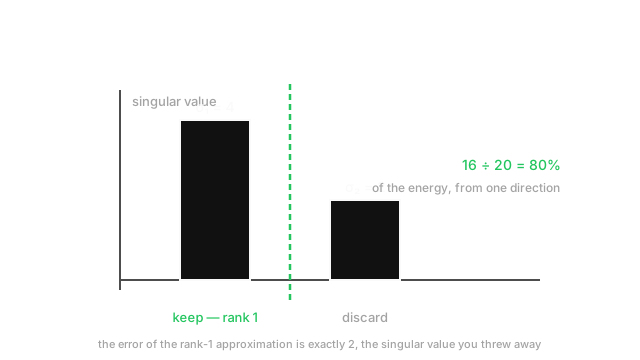
The Eckart–Young theorem is the guarantee that makes this useful: $A_k$ is the best rank- $k$ approximation of $A$ in both the Frobenius and spectral norms. No other rank- $k$ matrix is closer. And the error is exactly what you left out:

\lVert A - A_k \rVert_F = \sqrt{\sum_{i > k} \sigma_i^2}

So you can decide how much to discard before discarding it, by looking at the spectrum. The proportion of "energy" retained is $\sum_{i \le k} \sigma_i^2 / \sum_i \sigma_i^2$ , which is precisely the "explained variance" figure PCA reports.

The four uses worth knowing

PCA. Centre your data matrix, take its SVD, and the right singular vectors are the principal components while $\sigma_i^2/(n-1)$ are the explained variances. Doing it this way avoids forming $X^{T}X$ , which squares the condition number and loses precision.
Low-rank compression. Replace a weight matrix by its rank- $k$ truncation: storage drops from $mn$ to $k(m + n + 1)$ . LoRA is the same idea applied to the update rather than the weights.
Pseudo-inverse. $A^{+} = V \Sigma^{+} U^{T}$ , inverting only the nonzero singular values. This solves least squares even when the system is rank-deficient, which is what np.linalg.lstsq uses.
Conditioning. $\kappa = \sigma_1 / \sigma_r$ . Large means numerically fragile, and it is the honest way to check invertibility rather than a determinant.

Worked example

Take $A = \begin{bmatrix} 3 & 1 \\ 1 & 3 \end{bmatrix}$ — symmetric and positive definite, so its singular values equal its eigenvalues and everything is checkable by hand.

The characteristic polynomial is $(3-\lambda)^2 - 1 = 0$ , giving $\lambda = 4$ and $\lambda = 2$ . So $\sigma_1 = 4$ and $\sigma_2 = 2$ . Trace check: $3 + 3 = 6 = 4 + 2$ ✓. Determinant: $9 - 1 = 8 = 4 \times 2$ ✓.

The eigenvectors are $[1,1]$ and $[1,-1]$ , normalised to $u_1 = v_1 = \tfrac{1}{\sqrt{2}}[1,1]$ and $u_2 = v_2 = \tfrac{1}{\sqrt{2}}[1,-1]$ .

Now truncate to rank 1:

A_1 = \sigma_1 u_1 v_1^{T} = 4 \cdot \frac{1}{\sqrt 2}\begin{bmatrix} 1 \\ 1\end{bmatrix} \cdot \frac{1}{\sqrt 2}\begin{bmatrix} 1 & 1\end{bmatrix} = 4 \begin{bmatrix} 0.5 & 0.5 \\ 0.5 & 0.5 \end{bmatrix} = \begin{bmatrix} 2 & 2 \\ 2 & 2 \end{bmatrix}

The error:

A - A_1 = \begin{bmatrix} 1 & -1 \\ -1 & 1 \end{bmatrix}, \qquad \lVert A - A_1 \rVert_F = \sqrt{1+1+1+1} = 2

And 2 is exactly $\sigma_2$ , the singular value discarded — the Eckart–Young formula confirmed by hand.

Energy retained: $\sigma_1^2 / (\sigma_1^2 + \sigma_2^2) = 16/20 = 0.8$ . So one of two directions carries 80% of this matrix, which is the diagram's annotation.

Show Me the Code

1import numpy as np2
3A = np.array([[3.0, 1.0], [1.0, 3.0]])4
5U, s, Vt = np.linalg.svd(A)6print(s)                                        # -> [4. 2.]  sorted descending7print(np.allclose(A, U @ np.diag(s) @ Vt))       # -> True    reconstruction8
9A1 = s[0] * np.outer(U[:, 0], Vt[0])             # rank-1 truncation, shape (2, 2)10print(np.round(A1, 6).tolist())                  # -> [[2, 2], [2, 2]]11print(round(float(np.linalg.norm(A - A1)), 6))   # -> 2.0  == the discarded sigma12print(round(float(s[0] ** 2 / (s**2).sum()), 4)) # -> 0.8  energy kept13
14print(np.linalg.matrix_rank(A), round(s[0] / s[-1], 4))   # -> 2 2.0  rank, condition

Singular values 4 and 2, the rank-1 truncation [[2,2],[2,2]], error exactly 2, and 80% energy — every number matches the hand calculation.

Watch Out For

Running a full SVD when you only need the top few components

np.linalg.svd computes all singular values and vectors, at a cost of roughly $O(mn \cdot \min(m,n))$ . For a $100{,}000 \times 10{,}000$ matrix that is enormous, and if you wanted 50 components you have thrown almost all of it away.

Worse, the memory does not fit. A full $U$ for $m = 100{,}000$ is $100{,}000 \times 100{,}000$ — 40 GB in float32. This is the failure people hit first, and it is avoidable in one line: full_matrices=False returns the economy form, which is all anyone needs.

Beyond that, use a truncated solver. scipy.sparse.linalg.svds and sklearn.decomposition.TruncatedSVD compute only the top $k$ , and randomised SVD gets there faster still with accuracy that is fine for approximation work. For a sparse matrix this is not an optimisation but a requirement — a dense SVD densifies your sparse matrix first and exhausts memory.

The habit: decide $k$ before you decompose, then pick a routine that computes only $k$ .

Calling it PCA without centring the data first

PCA is the SVD of centred data. Skip the centring and the first component points toward the mean instead of along the direction of greatest variance, and every downstream number is quietly wrong.

The mechanism is easy to see. If your data sits in a tight cluster far from the origin — say all points near $(100, 100)$ — then the dominant direction in the uncentred matrix is the direction of that offset, because every row is roughly the same large vector. The genuine variation within the cluster is a small perturbation on top and shows up in later components, or not at all.

The symptom is a suspiciously dominant first component, often explaining 99%+ of "variance", followed by projections that all look the same. People interpret this as the data being one-dimensional when it is really just off-centre.

sklearn.decomposition.PCA centres for you; TruncatedSVD deliberately does not, because it is designed for sparse data where centring would destroy sparsity. Those two are not interchangeable, and swapping one for the other is a real and common bug. If you are calling np.linalg.svd directly, subtract the column means yourself, and keep them — you need them to project new data consistently.

The Quick Version

$A = U \Sigma V^{T}$ : rotate, scale, rotate. Works for any real matrix, and is always real.
Singular values are non-negative and sorted descending. All the distortion is in $\Sigma$ .
$\sigma_i = \sqrt{\lambda_i(A^{T}A)}$ , which is why SVD always exists. For symmetric positive definite matrices, singular values equal eigenvalues.
The count of nonzero singular values is the rank, so rank becomes a spectrum rather than a yes/no.
$A = \sum \sigma_i u_i v_i^{T}$ — a sum of rank-1 pieces ranked by importance.
Eckart–Young: the truncation $A_k$ is the best rank- $k$ approximation, and the error is $\sqrt{\sum_{i>k}\sigma_i^2}$ .
Energy retained $= \sum_{i \le k}\sigma_i^2 / \sum_i \sigma_i^2$ — this is PCA's explained variance.
Uses: PCA, low-rank compression and LoRA, the pseudo-inverse for rank-deficient least squares, the spectral norm, condition number $\sigma_1/\sigma_r$ .
Pass full_matrices=False, and use a truncated solver when you only want the top $k$ .
PCA requires centring. PCA centres, TruncatedSVD does not.