Core ML

Threshold Selection

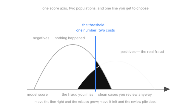
0.5 is a default that nobody chose. Put a price on each kind of mistake and the cut that minimises expected cost falls out as a ratio of those two prices.

Two overlapping score distributions share one axis, so wherever you put the cut you are choosing how many real positives to miss against how many clean cases to review

Why Does This Exist?

A card-fraud model scores each of the day's 200,000 transactions between 0 and 1. Somewhere a line of code turns that into a yes or a no, and in almost every codebase it reads score > 0.5. Nobody chose 0.5. It arrived as a library default and survived because it looked neutral.

It isn't. Move the line and two things trade against each other. A false positive is a clean transaction you flag: four minutes of review and a text the customer didn't need, call it two dollars. A false negative is fraud you wave through, an average chargeback of 180 dollars. Ninety times apart in price, and 0.5 treats them as identical. Same weights, same AUC — a different line, and the fraud team's day and the loss number both move.

One assumption throughout: the score means something. If 0.70 isn't a 70% chance, the arithmetic below is computing with something that isn't a probability, and probability calibration is what fixes that.

Think of It Like This

The sensitivity dial inside a smoke alarm

Open a smoke alarm and there's a sensitivity setting. Crank it up and the thing screams at burnt toast, so within a week somebody pulls the battery and you have no alarm at all. Crank it down and a real fire gets ninety seconds of head start.

No single setting is correct, and that's the point — it depends on the room. In a data centre a fire costs millions and a nuisance alarm costs a technician a walk down the hall, so you set it twitchy. Next to a bedroom, false alarms destroy the alarm, so you back it off and accept a slower response.

Same sensor, same physics, opposite settings, because the two mistakes cost different amounts in the two rooms. That is exactly the choice score > 0.5 makes for you, without asking which room you're in.

How It Actually Works

The arithmetic behind the cut

Let $C_{FP}$ be what a false positive costs — the two dollars of review — and $C_{FN}$ the 180-dollar chargeback. For a transaction the model scores at probability $p$ you have two options, each with an expected cost.

Flag it: you're wrong with probability $1 - p$ , so the cost is $(1-p) \, C_{FP}$ . Wave it through: you're wrong with probability $p$ , so the cost is $p \, C_{FN}$ . Flag whenever flagging is cheaper, and rearranging that comparison leaves one number:

t^{*} = \frac{C_{FP}}{C_{FP} + C_{FN}}

$t^{*}$ minimises expected cost, and notice what isn't in it: nothing about the model, nothing about the data, nothing about how rare fraud is. Just the ratio of the two prices. For 2 against 180 that's $2/182 = 0.011$ — eleven thousandths. Any problem where one mistake costs far more than the other lands nowhere near the middle.

The framings production actually uses

Expected cost is the honest framing when you can price both mistakes. Often you can't, and three alternatives each earn their place.

Maximise F-beta. It blends precision — of what you flagged, how much was fraud — with recall — of the fraud, how much you caught. $\beta$ sets how much more recall counts. Reach for it when recall clearly matters more and you can't name a price.

Hold a precision floor. "Reviewers disengage below 30% precision" is a real constraint, often the realest on the table. Take the lowest threshold that clears it, and read that off the precision-recall curve.

Fix an alert budget. The team reviews 200 a day, so send the top 200. That's a rank cut, not a probability cut, and it's what most deployed systems do — capacity is the binding constraint.

Where a threshold goes stale

Choose it on validation data, then leave it alone. It's a decision fitted to data like any other.

Then watch prevalence. Precision depends on the base rate as much as on the model: hold the threshold fixed, halve the fraction of fraudulent transactions, and precision roughly halves too. Reviewers see twice the noise and nothing in the code changed.

Which is the strongest practical argument for the alert budget. A rank cut says "the worst 200 today" and normalises itself — when scores drift up or down together, the top 200 is still the top 200. A probability cut says "everything above 0.011", and that moves with the score distribution.

Show Me the Code

Same model, five different lines, and the cost swings by a factor of six.

1import numpy as np2
3COST_FP, COST_FN = 2.0, 180.0    # four minutes of a reviewer vs an average chargeback4
5
6def cost_at(p: np.ndarray, y: np.ndarray, t: float) -> float:7    flag = p >= t8    return float(COST_FP * (flag & (y == 0)).sum() + COST_FN * (~flag & (y == 1)).sum())9
10
11rng = np.random.default_rng(11)12p = rng.beta(0.6, 12.0, 200_000)            # a calibrated score, base rate near 5%13y = (rng.random(200_000) < p).astype(int)   # so the outcome really happens at rate p14
15for t in (0.50, 0.20, 0.05, COST_FP / (COST_FP + COST_FN), 0.004):16    print(f"cut {t:.4f}   flagged {(p >= t).sum():6d}   cost {cost_at(p, y, t):,.0f}")17# -> cut 0.5000   flagged     23   cost 1,719,20618# -> cut 0.2000   flagged   5805   cost 1,454,85819# -> cut 0.0500   flagged  65754   cost 500,59220# -> cut 0.0110   flagged 137085   cost 298,72821# -> cut 0.0040   flagged 164588   cost 318,608

The minimum lands on 0.0110, which is $C_{FP}/(C_{FP}+C_{FN})$ to four places, and it beats 0.5 by 1.42 million. Overshoot to 0.004 and cost climbs again, so the curve really has a bottom.

Now read the other column. The cost-optimal cut flags 137,085 of 200,000 transactions, and no review team absorbs that. Either the score is too diffuse, or the real constraint was never cost but capacity.

Watch Out For

Tuning the threshold on the test set

You sweep 200 thresholds, pick the best F2, and report that F2. It reads as a measurement. It's the maximum of 200 noisy numbers, and a maximum over noise is biased upward by construction.

Choosing a threshold is model selection, so it belongs on validation data. Pick the cut there, then evaluate that frozen cut once on test. On a small test set the gap is large, and it's the gap that becomes a surprise the week after launch. Train, validation and test splits covers the plumbing.

Shipping a threshold and never revisiting it

The threshold was right in March. By September the fraud mix has shifted, an upstream feature changed units, and the score distribution has slid left. Recall is down eight points, precision down six. No deploy happened and no test failed — every gate in the pipeline compares the model to itself.

Track flagged volume and the precision of the flagged set on a rolling window, and alert when either leaves its band — volume moves first. Then re-fit the cut on recent labels on a schedule, rather than after a complaint. Data drift and distribution shift is the wider version, and a rank-based budget absorbs much of it for free.

The Quick Version

0.5 is a library default, not a decision. It assumes both mistakes cost the same.
With a calibrated score and two prices, the expected-cost-minimising cut is $C_{FP}/(C_{FP}+C_{FN})$ , and nothing about the model appears in it. For 2 against 180 that's 0.011.
Can't price both mistakes? Maximise F-beta, hold a precision floor, or fix an alert budget and take the top N — that last one is what most deployed systems use, because capacity is the constraint that doesn't move.
Pick the cut on validation data. Tuning it on test is model selection in disguise.
Precision moves with prevalence at a fixed threshold, so a probability cut decays where a rank cut doesn't.