Data Concepts

Missing Data

A blank cell is a fact about how your data was collected, not an absence of information. Why the value is gone decides what you're allowed to do about it.

Three reasons a cell is blank: nothing points at the gap, a column you already have points at it, or the missing value points at itself, and only that last one cannot be settled from the data you hold

Why Does This Exist?

A survey lands with 4,000 rows and an income column that is 22% blank. df.dropna() leaves 3,120 rows, the model trains without a warning, and every metric looks reasonable.

You have just fitted a model to the people who were willing to state their income. That is not the population anyone asked you about, and no validation score will tell you.

A blank cell is a record of something that happened during collection. A sensor lost power. A field was optional. A question got skipped by 22% of people for a reason. The value is gone; the reason is often still sitting in your data, and whether it is decides what you're allowed to do next.

So the useful question is never "what do I fill this with". It's why is it blank — and the three possible answers behave so differently that they have their own names.

The vocabulary, in one paragraph

Missingness is usually described as a mask: a second table the same shape as your data, holding a one where a value is present and a zero where it's blank. The missingness mechanism is the causal story behind that mask. Listwise deletion — what dropna() does — discards any row with a blank anywhere in it. Imputation replaces the blank with a guess. A missingness indicator is a new column recording where the blanks were, so a model can use their positions as evidence.

Think of It Like This

Three ways a page goes missing from a filing cabinet

You inherit a cabinet of patient files. Pages are missing. Before you can say anything about the patients, you have to work out how pages left.

Someone knocked coffee into a drawer and a random handful of pages were binned. Nothing about a page made it more likely to go. What survived is a fair sample of what was there.

The Wednesday clinic had a temp clerk who never filed anything. Pages are gone in a pattern, but the pattern is written on the folders you still have: every file records which day it came from. Knowing the day, you can reason about what left.

Some patients read their own notes and tore out the page they were embarrassed by. Now the reason a page is gone is the thing that was printed on it. Study the surviving pages as long as you like — they cannot tell you what the torn ones said, because being torn is what removed them from view.

Same cabinet, same visible gap, three completely different situations. And the cabinet itself cannot tell you which of the last two you're in. Only the clerk can.

How It Actually Works

Write $M$ for that mask of ones and zeros, $X_{\text{obs}}$ for the values you can see, and $X_{\text{mis}}$ for the values you can't. The three mechanisms differ in what the mask depends on:

\text{MCAR}: P(M) \qquad \text{MAR}: P(M \mid X_{\text{obs}})\qquad \text{MNAR}: P(M \mid X_{\text{mis}})

Read left to right, that says: the gaps are unrelated to everything, the gaps depend on columns you have, the gaps depend on the values you don't have.

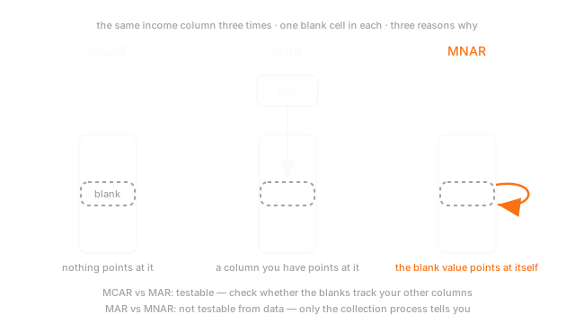
MCAR — missing completely at random. A sensor dropped a packet. A row got truncated by a bad export. Nothing about the record makes it likelier to be blank. Deletion here costs sample size and nothing else, which is why MCAR is the assumption everyone quietly makes and almost nobody has.

MAR — missing at random. Older patients skip the online form, and you have age. The name misleads: the gaps are anything but random, they're just explainable by columns already in your table. That's the workable case, because a model of the observed columns can stand in for what left.

MNAR — missing not at random. High earners decline to state income. The probability of the blank depends on the number that would have been in it. This is the one that hurts, and no imputation fixes it, because the evidence you'd need is precisely what's absent.

What you can and cannot test

You can test MCAR against MAR. Build the indicator column — one for blank, zero for present — and check whether it relates to anything you observe: group means, a correlation, or a small classifier predicting the indicator from the other columns. If income_missing runs 3% among under-30s and 34% among over-65s, the gaps track age. Not MCAR. Settled, from data alone.

You cannot test MAR against MNAR. Both stories predict the same observed table. Separating them needs a fact about collection — who asked, whether the question was skippable, whether the sensor saturates at its ceiling — and that fact lives with the people who built the pipeline, not in the file they handed you. Ask them. It's the highest-value 20 minutes in the whole cleaning task.

The indicator column is nearly free

Whatever you do about the value, keep the fact that it was absent:

1income        income_missing2 42000        03   NaN        1

Under MAR it lets a model recover part of what deletion would have thrown away. Under MNAR it's often the most predictive thing in the row — a customer who won't share income behaves differently, and "declined to answer" is signal, not a defect. Under MCAR it costs one column the model will ignore. Every branch of that is fine.

Three shapes the gaps take

Univariate — one column carries all the blanks, so everything above applies to it directly.

Monotone — once a row goes blank it stays blank, the staircase you get from dropout. Weeks 1 to 4 are full, week 5 has gaps, week 6 has those plus more. Cohort studies and app retention both look like this, and the staircase itself is data about who left.

Arbitrary — blanks scattered across many columns with no structure. Most real tables, and where deletion turns brutal for the reason below.

Worked example

Eight people, income in thousands: 20, 24, 28, 32, 36, 40, 60, 120. The mean is $360/8 = 45$ .

Now make it MNAR: the two highest earners decline to state. Six rows survive, they sum to 180, and dropna() reports a mean of $180/6 = 30$ .

The bias isn't random. It points down, by 15, and you can compute it in advance if you know which end went. The median moves too, from 34 to 30, but only by one position's worth — the same mean-versus-median gap from descriptive statistics, showing up as a reason to distrust a deleted mean in particular.

Show Me the Code

1import numpy as np2
3income = np.array([20.0, 24.0, 28.0, 32.0, 36.0, 40.0, 60.0, 120.0])4declined = np.array([0, 0, 0, 0, 0, 0, 1, 1], dtype=bool)  # MNAR: the top two opt out5
6
7def dropna_mean(values: np.ndarray, blank: np.ndarray) -> float:8    """What listwise deletion reports: the mean of whatever survived."""9    return float(values[~blank].mean())10
11
12print(income.mean(), dropna_mean(income, declined))     # -> 45.0 30.013print(np.median(income), np.median(income[~declined]))  # -> 34.0 30.014print(round(0.9**5, 5))   # -> 0.59049   five columns, 10% blank each, at random

That last line is the arithmetic behind the first pitfall, and it surprises people every time.

Watch Out For

Reaching for dropna() by reflex

Deletion feels neutral. It isn't, and it fails in two separate ways.

The first is bias. Under MAR or MNAR, the rows you keep are a different population from the rows you started with, so every statistic you compute afterwards answers a question nobody asked. The worked example above lost 15 units of mean income to a mechanism you could name.

The second is volume, and it's the one that catches people off guard. Blanks scattered across columns compound multiplicatively. Five columns, each 10% blank independently, and the fraction of rows with no blank anywhere is $0.9^5 = 0.59$ . You just deleted 41% of your data. Ten such columns leaves 35%. Nobody looks at a table with 10% missing per column and expects to lose a third of it.

Deletion is defensible in one case: you have solid reason to believe MCAR, and you can afford the rows. Otherwise keep the row, keep an indicator, and choose an imputation you can justify.

Sentinel values that read as real magnitudes

-1, 0, 999, -9999, 1900-01-01, the empty string, "N/A". Someone upstream needed a non-null value in a non-null column, so they picked one. Nothing in the file marks it as special.

Downstream, a model sees numbers. An age of -1 is not a gap to it; it's a person 41 years younger than a 40-year-old. Take 1,000 rows where the 800 real ages average 40 and the other 200 hold -1, and the column mean is $(800 \times 40 - 200)/1000 = 31.8$ . Your scaler is now fitted to that. Your tree splits on it. The zero-coded ones are worse, because zero is plausible for counts and spend, so no plot looks wrong.

Two habits. Ask the source system what its null convention is, before you read the data. Then check every numeric column's min, max and most frequent value — sentinels sit at the extremes or pile up in one bin, and value_counts() on the tails finds them fast. Convert them to real nulls before anything is fitted.

The Quick Version

A blank cell is evidence about collection. Ask why it's blank before you ask what to put there.
MCAR: the gap relates to nothing. MAR: it depends on columns you have. MNAR: it depends on the value that's gone.
You can test MCAR against MAR from data — predict the missingness indicator from the other columns and see if it works.
You cannot separate MAR from MNAR from data. That needs someone who knows the collection process.
MNAR is the dangerous one, because the evidence needed to correct it is exactly what's absent.
Keep a missingness indicator regardless. One column, and under MNAR it's often the most predictive thing in the row.
Patterns: univariate, monotone (dropout), arbitrary. Arbitrary is the common one and the worst for deletion.
dropna() biases the population and costs more rows than you expect: five columns at 10% each keeps 59%.
Sentinels like -1 and 999 are gaps wearing the clothes of measurements. Hunt them before you fit anything.