Data Concepts

Text Feature Representation

Counting words gets you a strong baseline in seconds. TF-IDF weights each count by how rare the token is, and that weighting is most of the whole trick.

Three documents become a document-term matrix where nearly every cell is zero, and TF-IDF gives its highest weight to the one token unique to a single document

Why Does This Exist?

A model wants a fixed-width row of numbers. A document is a variable-length string. The oldest bridge between them still works: count the words.

Take a position here, because plenty of teams don't. Run a TF-IDF plus linear baseline before any transformer. It trains in seconds, tells you which token drove which prediction, and beats a badly-tuned embedding pipeline more often than anyone writes up. On short reviews, tickets and spam the gap to a fine-tuned encoder is often a couple of points of F1, sometimes the wrong way round.

Think of It Like This

Telling dishes apart from the shopping list

Someone hands you two shopping lists. No recipe, no method — just what went in each basket.

List one: flour, butter, sugar, four eggs, vanilla. List two: onions, garlic, ginger, cumin, coriander, turmeric, chicken, rice.

You knew which was a cake before you finished reading, and word order never came into it.

Now look at which ingredients did the work. Salt would have told you nothing; turmeric told you almost everything, because it turns up in so few other baskets. Rarity carries the signal — that's the whole of TF-IDF.

Where the list fails: it has no order, so "not very good" and "very good" arrive nearly identical.

How It Actually Works

Counts first, then weights

Bag of words. Fix a vocabulary from your training documents, one column per token; each document becomes a vector of counts. Bag-of-words discards word order by construction — "the dog bit the man" and "the man bit the dog" give identical rows.

N-grams. Treat adjacent pairs as columns of their own, so not good becomes a feature and local order comes back. The bill is vocabulary size: 50,000 unigrams can become millions of columns once bigrams are in.

TF-IDF. Raw counts overweight what's common, and what's common is mostly grammar. So reweight each count by how rare the token is across documents:

\text{tfidf}(t, d) = \text{tf}(t, d) \times \log\frac{N}{1 + \text{df}(t)}

Every symbol: $t$ is a token, $d$ one document, $\text{tf}(t, d)$ how many times $t$ appears in $d$ , $N$ the number of documents in the corpus, $\text{df}(t)$ the document frequency — how many of those $N$ documents contain $t$ at least once — and $\log$ the natural logarithm. The $+1$ keeps the fraction finite for a token never seen.

Frequent here and rare elsewhere gives a large $\text{tf}$ times a large log, so it scores highest. A token in every document has $\text{df} \approx N$ , so the fraction lands near 1 and the log near 0: at 10,000 documents with $\text{df} = 10{,}000$ the weight is $-0.0001$ . Grammar cancels itself.

L2 row normalisation. A 2,000-word document has larger counts than a 40-word one, so length alone would dominate every distance. Divide each row by its L2 norm and each document becomes a unit vector, which makes the dot product a cosine.

The hashing vectoriser. Hash each token into one of $k$ buckets you pick instead of learning a vocabulary. Fixed width before you see data, no fit, and it streams. You give up the inverse mapping: no coefficient reads back as a word.

What none of this can do

No synonymy. car and automobile are separate columns, orthogonal to each other — cosine similarity exactly zero.
No order past the n-gram window. Bigrams catch not good, not a negation five words upstream.
No unseen tokens. A word absent from the training vocabulary is dropped in silence; a document of all-new words becomes an all-zero row, scored anyway.
A vocabulary that grows with the corpus. The matrix widens as it gets taller — the door into sparse data and high dimensionality.

The knobs that matter

min_df drops tokens appearing in fewer than n documents and is the highest-value setting here — min_df=2 often removes half the vocabulary, nearly all of it typos. max_df=0.9 drops near-universal tokens. sublinear_tf=True swaps $\text{tf}$ for $1 + \log \text{tf}$ . Stopwords are a decision: strip not from sentiment text and the task is gone.

Worked example

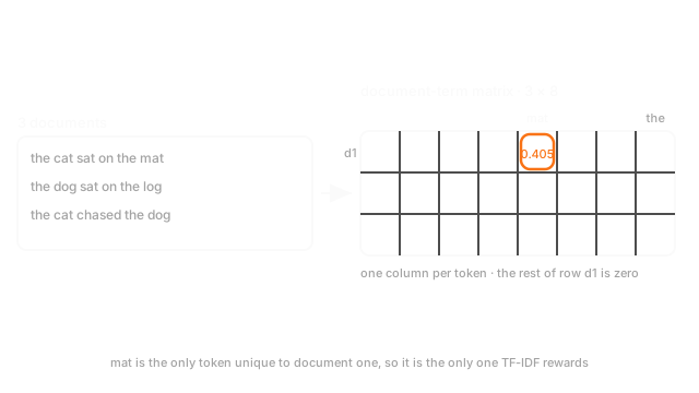
Three documents: $d_1$ "the cat sat on the mat", $d_2$ "the dog sat on the log", $d_3$ "the cat chased the dog". The sorted vocabulary is 8 columns — cat, chased, dog, log, mat, on, sat, the — so $N = 3$ , the sits in all three and mat in one.

Take mat in $d_1$ , where $\text{tf} = 1$ and $\text{df} = 1$ :

1 \times \log\frac{3}{1 + 1} = \log 1.5 = 0.405

the appears twice with $\text{df} = 3$ , so $2 \times \log(3/4) = -0.575$ . cat, at $\text{df} = 2$ , gets exactly $0$ . mat wins — the only token in $d_1$ above zero, and the one no other document has. Those negatives and hard zeros are an artefact of three documents.

Show Me the Code

1import numpy as np2
3docs: list[list[str]] = [4    ["the", "cat", "sat", "on", "the", "mat"],5    ["the", "dog", "sat", "on", "the", "log"],6    ["the", "cat", "chased", "the", "dog"],7]8vocab: list[str] = sorted({w for d in docs for w in d})9
10
11def tf_idf(corpus: list[list[str]], terms: list[str]) -> np.ndarray:12    tf = np.array([[d.count(w) for w in terms] for d in corpus], dtype=float)13    df = (tf > 0).sum(axis=0)                        # documents containing each token14    return tf * np.log(len(corpus) / (1 + df))       # the +1 keeps an unseen token finite15
16m = tf_idf(docs, vocab)17print(round(float(m[0, vocab.index("mat")]), 3))     # -> 0.405   unique to document one18print(round(float(m[0, vocab.index("the")]), 3))     # -> -0.575  in all three, so cancelled19print(vocab[int(m[0].argmax())])                     # -> mat

df is counted across whatever corpus you pass in — hence the first pitfall below.

Watch Out For

Fitting the vectoriser on the whole corpus

vectorizer.fit_transform(all_documents), then a split. One line shorter than the correct order, so it's everywhere.

Two things crossed the boundary: the vocabulary now holds tokens that only appear in test documents, and the document frequencies were counted over them too, so every $\text{idf}$ in your training matrix knows about the held-out set.

It bites harder than a numeric scaler because text vocabularies are long-tailed: a rare token in three test documents and none of the training ones gets a big $\text{idf}$ and a column of its own. Scores get inflated this way routinely.

Fit on training documents, transform the rest, and put the vectoriser in a Pipeline. See data leakage and train, validation and test splits.

Calling .toarray() on a document-term matrix

Someone hands the matrix to an estimator that wants dense input, and reaches for .toarray().

Do the arithmetic. 150,000 documents, a 200,000-token vocabulary, 50 distinct tokens each. As a sparse matrix in CSR that's about 7.5 million non-zeros, so around 90MB. Dense float64 is $150{,}000 \times 200{,}000 \times 8$ bytes: 240GB. You asked a 16GB laptop for 240GB, and it either swapped until the kernel died or raised MemoryError.

Subtracting a column mean does the same damage without the honest crash. To inspect, slice first — m[:5].toarray() is 8MB. To scale, StandardScaler(with_mean=False) or MaxAbsScaler.

The Quick Version

Run TF-IDF plus a linear model before any transformer: seconds to train, readable per token, a real number to beat.
Bag of words is counts over a fixed vocabulary, order discarded on purpose. N-grams buy order back at the cost of width.
$\text{tf} \times \log(N / (1 + \text{df}))$ : frequent here and rare elsewhere scores highest; present everywhere scores near zero.
L2-normalise rows, or length dominates. Hashing trades the token mapping for fixed width.
No synonymy, no long-range order, no way to handle an unseen token.
min_df=2 is the highest-value setting; stopwords are a decision, not a default.
Fit on training documents only, and keep it sparse: 240GB dense versus 90MB in CSR is the same matrix.