Gen AI

Autoregressive Image Generation

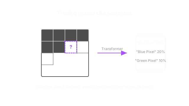
Instead of starting with static and slowly denoising an entire image at once, an autoregressive model starts at the top-left corner and generates the image one pixel at a time, reading it exactly like a book.

Autoregressive image models predict an image sequentially, one patch at a time, exactly like an LLM predicting the next word in a sentence.

Why Does This Exist?

When the Transformer architecture (the backbone of ChatGPT) was released, researchers realized it was unbelievably good at scaling. The more data and compute you threw at a Transformer, the smarter it got. Naturally, researchers wanted to use Transformers for image generation, long before Diffusion Transformers (DiTs) existed.

Large Language Models (LLMs) are autoregressive. This means they predict a sentence one word at a time based on all the previous words. Researchers asked a crazy question: "Can we just treat an image like a sentence?" If you flatten a 2D image into a 1D sequence of pixels, can an LLM just predict the next pixel?

The answer was yes. Autoregressive Image Generation models (like Google's Parti or OpenAI's original ImageGPT) proved that the exact same architecture used to write essays could also paint photorealistic pictures, simply by changing the vocabulary from "words" to "colors."

Think of It Like This

The Typewriter Artist

Imagine an artist using a typewriter to create a picture out of colored letters.

Diffusion Models: The artist throws down a sheet of paper covered entirely in random, messy ink splotches. They spend an hour slowly wiping away the ink with a sponge until a beautiful image is left behind.
Autoregressive Models: The artist rolls a blank sheet of paper into the typewriter. They look at the prompt, hit a red key for the top-left pixel, move the carriage one space, hit a blue key for the next pixel, and proceed row by row, left to right, top to bottom, until the image is perfectly typed out.

How It Actually Works

Autoregressive models reframe image generation from a continuous physics problem (like diffusion) into a discrete classification problem (like text generation).

1. The Vocabulary of Pixels

An LLM uses a vocabulary of about 50,000 "tokens" (sub-words). To make an LLM generate images, we need an image vocabulary. A naive approach is to use the 256 values of RGB as the vocabulary. However, a 1024x1024 image has over 3 million color values. A Transformer trying to predict 3 million tokens in a row would take days to generate a single image and would run out of RAM instantly.

2. VQ-VAEs (Vector Quantization)

To solve the sequence length problem, researchers use a specialized autoencoder called a VQ-VAE (Vector Quantized Variational Autoencoder). Instead of compressing the image into continuous math (like standard Latent Diffusion), the VQ-VAE compresses an 8x8 block of pixels into a single, discrete ID number from a "codebook." For example, ID #42 might mean "a patch of furry texture," and ID #800 might mean "a sharp metallic edge." By converting the image into these discrete patches, the sequence length drops from 3,000,000 pixels down to just 1,024 tokens.

3. Next-Token Prediction

Now, the image is just a sequence of numbers: [42, 800, 15, 99...]. We feed this exact sequence into a standard, decoder-only Transformer (the exact same architecture as GPT-4). We train it using standard Cross-Entropy Loss: "Given the text prompt and the past 50 image tokens, predict the 51st image token."

4. Inference

To generate an image, you give the model a text prompt. It predicts the first patch. It appends that patch to its context, then predicts the second patch. It repeats this 1,024 times. Finally, you pass the generated sequence of 1,024 tokens back through the VQ-VAE decoder to turn the IDs back into a high-resolution, photorealistic image.

Show Me the Code

This pseudocode shows the incredibly simple inference loop of an autoregressive image generator. Notice how it is completely identical to a text generation loop.

1import torch2
3def generate_image_autoregressively(transformer, vq_vae, text_prompt, sequence_length=1024):4    """5    Generates an image one patch at a time.6    """7    # 1. Encode the text prompt into the model's context8    context = encode_text(text_prompt) 9    10    # We start with an empty sequence of image tokens11    generated_tokens = []12    13    # 2. Generate the sequence one token at a time14    for _ in range(sequence_length):15        # The transformer looks at the text and the tokens generated SO FAR16        # and outputs probabilities for the NEXT token across the vocabulary (e.g., 8192 codes)17        logits = transformer(context, generated_tokens)18        19        # Sample the most likely next patch ID (e.g., ID #405)20        next_token = sample_from_logits(logits)21        22        generated_tokens.append(next_token)23        24    # 3. We now have a full list of 1024 token IDs. 25    # Use the VQ-VAE to decode these IDs into actual RGB pixels.26    image_tensor = torch.tensor(generated_tokens)27    final_image = vq_vae.decode(image_tensor)28    29    return final_image

Watch Out For

The Unidirectional Blind Spot

Because autoregressive models predict strictly from top-left to bottom-right, they suffer from a "unidirectional blind spot." When predicting a pixel in the middle of the image, the model cannot look ahead to see what the bottom-right corner looks like, because it hasn't generated it yet. This can sometimes lead to structural inconsistencies (like a building that makes sense at the top but abruptly changes architecture at the bottom) compared to diffusion models, which evaluate the entire image globally at every step.

The Quick Version

Autoregressive image models treat images exactly like sentences, generating them one piece at a time from top-left to bottom-right.
Because generating millions of raw pixels is computationally impossible for Transformers, the images are first heavily compressed into a "vocabulary" of discrete patches using a VQ-VAE.
The model uses the exact same next-token prediction math (Cross-Entropy Loss) as ChatGPT.
While they benefit immensely from LLM scaling laws, their sequential nature makes inference much slower than single-step diffusion models, and their unidirectional generation can sometimes cause global layout issues.