Flow Matching
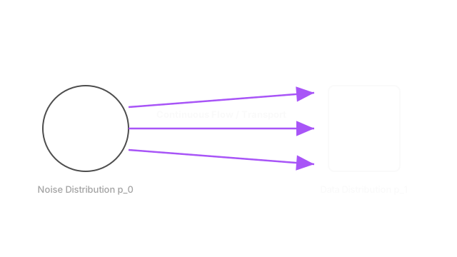
Flow matching replaces the confusing math of standard diffusion models by simply drawing a straight line between pure noise and a real image, and teaching a neural network to walk down that line.
Why Does This Exist?
Denoising Diffusion Probabilistic Models (DDPMs) and Score-Based Models revolutionized generative AI, but they arrived with an immense amount of mathematical baggage. They required complex variance schedules, Fokker-Planck equations, and Langevin dynamics to explain what was fundamentally a simple concept: gradually turning noise into data.
Worse, the path a standard diffusion model takes from noise to data is heavily curved and inefficient. Flow Matching was introduced as a simpler, more elegant alternative that strips away the stochastic baggage. Instead of relying on a random Markov chain, Flow Matching defines a deterministic, straight-line path (an Ordinary Differential Equation, or ODE) directly from a noise sample to a data sample. This makes the math vastly easier to understand, the training more stable, and the generation significantly faster because straight lines are easier for numerical solvers to simulate than curved ones.
Think of It Like This
The Crowd in the Field
Imagine 1,000 people standing completely randomly in a giant square field (the Noise Distribution). Suddenly, you tell them to form a perfect circle in the center of the field (the Data Distribution).
- Diffusion Models: Everyone wanders around semi-randomly, bumping into each other, slowly drifting toward the center over an hour until they eventually form the circle. It works, but it's chaotic.
- Flow Matching: Every single person looks at exactly where they need to stand in the circle, draws a straight line in the dirt from their current spot to their target spot, and walks forward at a constant speed. It is direct, deterministic, and optimally efficient.
How It Actually Works
Flow Matching unifies concepts from Continuous Normalizing Flows (CNFs) and Optimal Transport into a highly trainable framework.
1. Defining the Vector Field
In a generative model, we want to map a simple distribution (like a standard Gaussian noise) to a complex distribution (like real images). We can do this by defining a continuous transformation over time from to . To move the probability mass from to , we need a vector field that tells us which direction to push a particle at any time . If we have this vector field, we can just use an ODE solver to push noise particles until they become images.
2. The Flow Matching Objective
Historically, training a neural network to learn this vector field directly was computationally impossible because it required simulating the entire flow path (using something called Neural ODEs). The breakthrough of Flow Matching is the realization that if we know the start point (a specific noise sample ) and the end point (a specific image ), we can just define the vector field for that specific pair! We draw a straight line between them. The target vector field is simply .
We then train a neural network to predict this target vector field. The loss function is a simple Mean Squared Error between the network's prediction and the straight-line target .
3. Simulation-Free Training
Because we already know the target vector field , we don't have to simulate the ODE during training. We just sample a random time , interpolate between the noise and the image (e.g., ), and ask the network to predict the direction . This is called "simulation-free" training, and it is exactly what makes DDPMs scale so well, now applied to a much cleaner mathematical framework.
4. Generation
During inference, we sample pure noise . We then use an ODE solver (like Euler's method) to follow the learned vector field . Because Flow Matching paths are inherently much straighter than standard diffusion paths, ODE solvers can take much larger steps without making errors, resulting in high-quality generation in far fewer steps (e.g., 5 to 10 steps instead of 50).
Code
This code demonstrates the elegantly simple training objective of a Flow Matching model. Notice how there are no complex schedules or cumulative variances compared to a DDPM.
import torchimport torch.nn as nn
def flow_matching_training_step(model: nn.Module, x_1: torch.Tensor) -> torch.Tensor: """ Computes the Flow Matching loss for a single training step. Args: model: The network predicting the vector field. x_1: Clean batch of images (B, C, H, W). """ # 1. Sample pure noise (x_0) x_0 = torch.randn_like(x_1) # 2. Sample a random time t between 0 and 1 t = torch.rand(x_1.shape[0], 1, 1, 1, device=x_1.device) # 3. Interpolate along a straight line # x_t is a mixture of noise and data x_t = (1 - t) * x_0 + t * x_1 # 4. The target vector field is simply the straight line direction target_v = x_1 - x_0 # 5. The model predicts the vector field at x_t predicted_v = model(x_t, t.squeeze()) # 6. Mean Squared Error loss loss = nn.functional.mse_loss(predicted_v, target_v) return loss
# Example usage# loss = flow_matching_training_step(vector_field_network, real_images)Watch Out For
Optimal Transport is Hard
While we pair a random noise sample with a random image , this random pairing causes crossing paths. If Noise Particle A is paired with Cat Image B, and Noise Particle C is paired with Dog Image D, their straight lines might cross. When paths cross, the vector field becomes ambiguous, forcing the neural network to average the directions, which results in blurry generations. Advanced techniques (like Optimal Transport Flow Matching or Rectified Flow) sort the noise/image pairs to minimize the distance they have to travel, preventing paths from crossing and producing much sharper results.
The Quick Version
- Flow Matching is a modern alternative to standard diffusion models that uses Ordinary Differential Equations (ODEs) instead of stochastic Markov chains.
- Instead of complex noise schedules, it trains a neural network to learn a vector field that transports a noise distribution directly to a data distribution.
- The training objective is remarkably simple: pair a noise sample with an image, draw a straight line between them, and penalize the network if it doesn't predict that straight-line direction.
- Because the learned paths are straight, inference is significantly faster and requires fewer steps than standard diffusion models.
- Flow Matching is rapidly becoming the foundation for the next generation of text-to-image and text-to-audio models due to its simplicity and efficiency.